The duration of features

Geometric vector features on their own do not say much about plate tectonic evolution, they just represent the spatial extent of units as points, lines or polygons. In themselves they only have durations.

Load in the plate polygons by going to File->Open Feature Collection…, navigate to GeoData/FeatureCollections/ContinentalPolygons and open Global_EarthByte_GPlates_PresentDay_ContinentalPolygons.gpmlz!

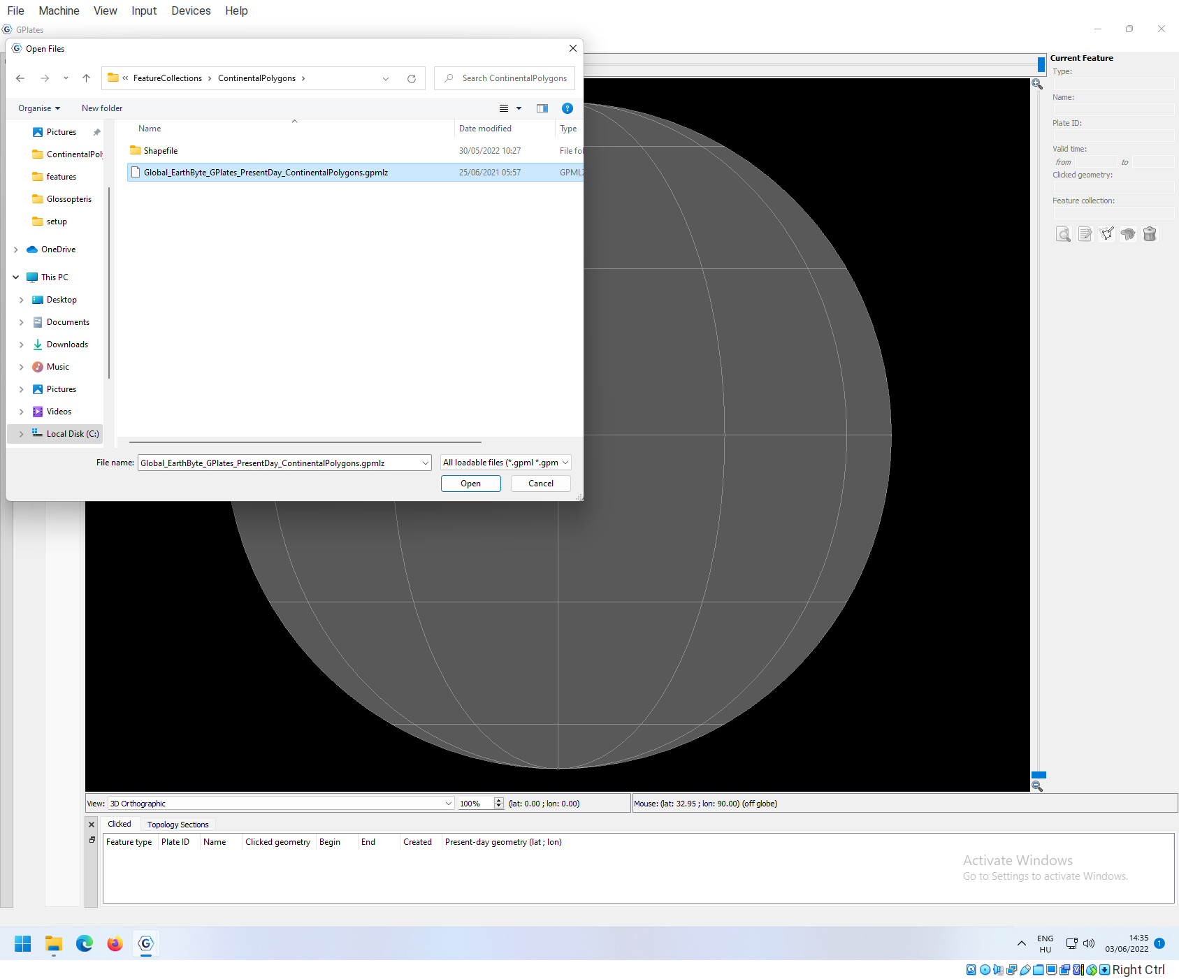
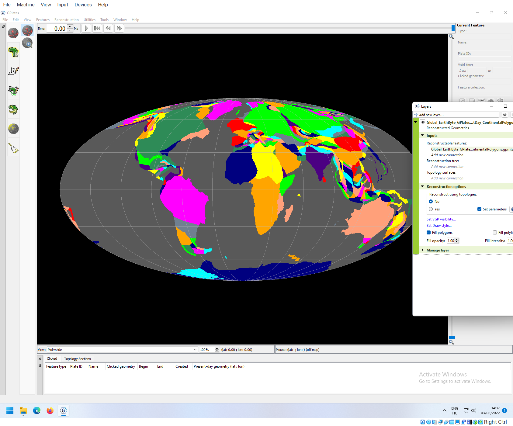
Note that after you load in the feature collection, if the time is set to 0, you can see all polygons: (view set to Mollweide projection, and polygons are filled)

If you move the time slider back (e.g. to 200Ma), you will note that some polygons are disappearing.

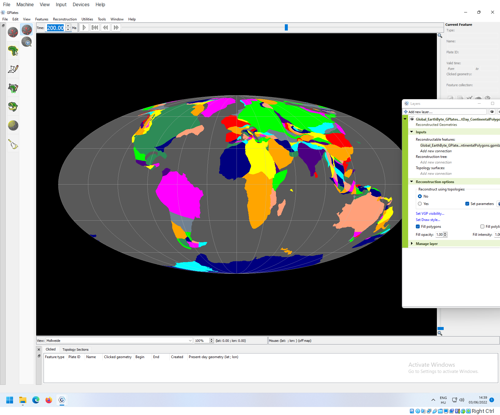
Note where this happens, and go back to the present day to see these polygons. You can use the Inspect features tool to see the attributes of such polygons:

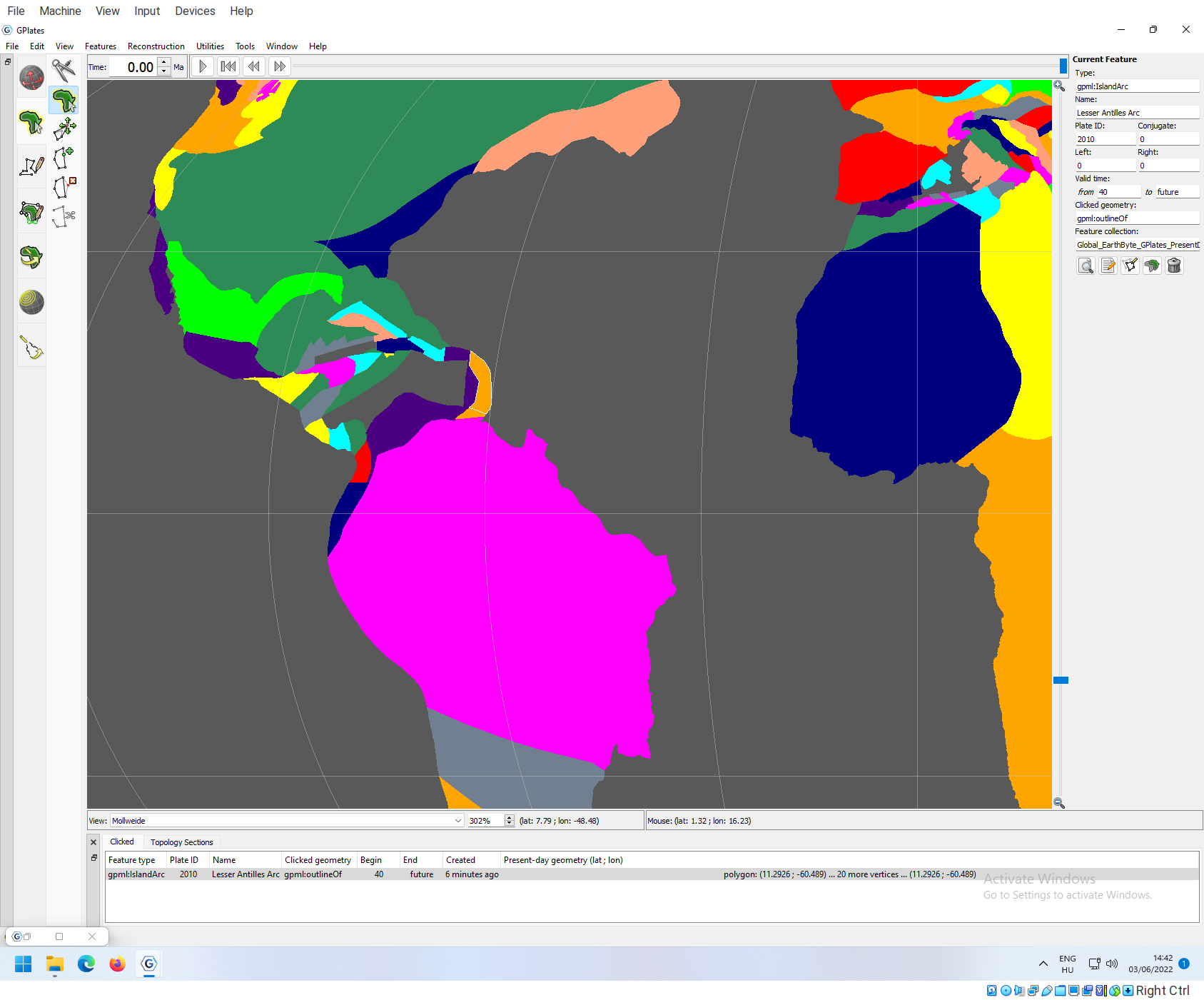
If you lookat the right-hand side panel, you will see that there are entries for Valid time that range from a value to another value. In the case of the selected Lesser Antilles Arc, the from value is set to 40 (Ma), and the to is set to future, which means that this feature starts to exist only at 40Ma, and it will not disappear in the future. If the reconstruction time moves beyond the interval outlined by these two values, the feature will not be included in that reconstruction.

These values set whether features exist or not at a time, but they do not move them around. For that we need rotation files. You can go ahead and unload/eject the Continental Polygons feature now.

Rotations

Download example

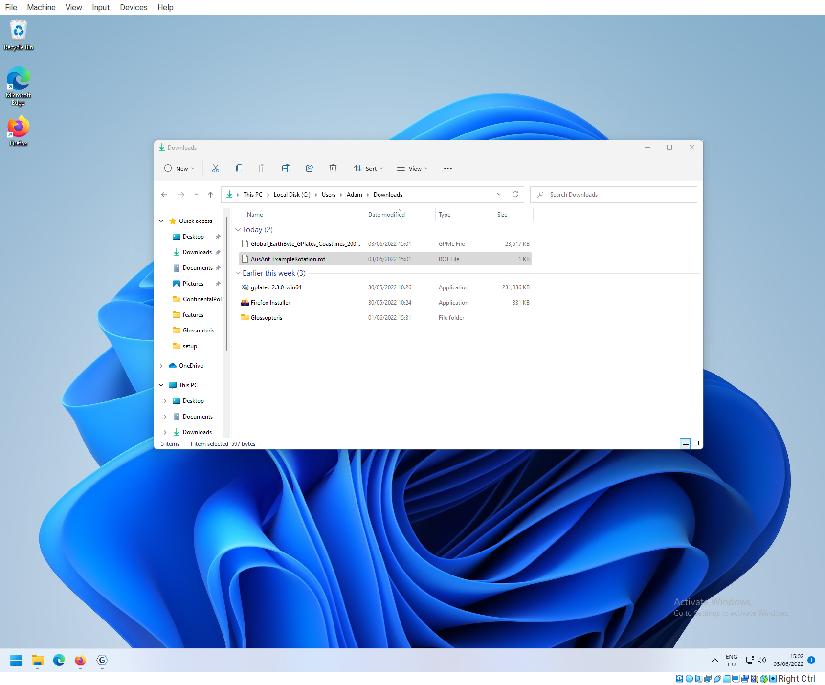
To better understand what is actually happening in such a model, we need to simplify a complete plate tectonic reconstruction to the elemental baseics. For this exercise, go on and download these example files

and put them in a convenient folder (in this case they will be in the Downloads folder).

Example Coastlines

You can open the coastlines file with the Open Feature Collection tool.

You can use the inspect tool to confirm that the following features have these Plate IDs:

Feature	Plate ID
Africa	701
Australia	801
Antarctica	802
Tasmania	850

The rotation file

To see how rotations work, we are going to implement a single rotation, and add it to an already structured file. The rotation file has .rot extension. It is a plain text file that can be opened by any text or code editor.

Opening the rotation file in Notepad

Go on an open this file in notepad (Windows’ default text editor), by 1. navigating to the file in Windows Explorer, 2. right click on the file, and select Open with:

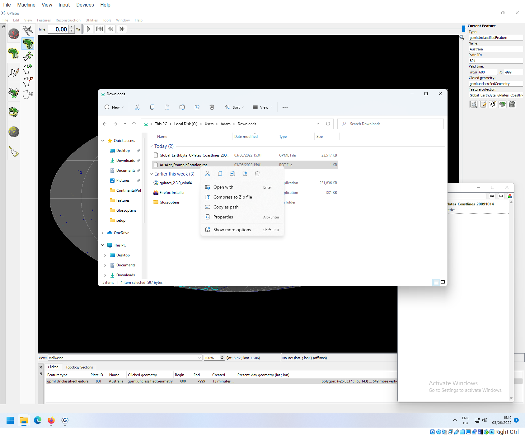
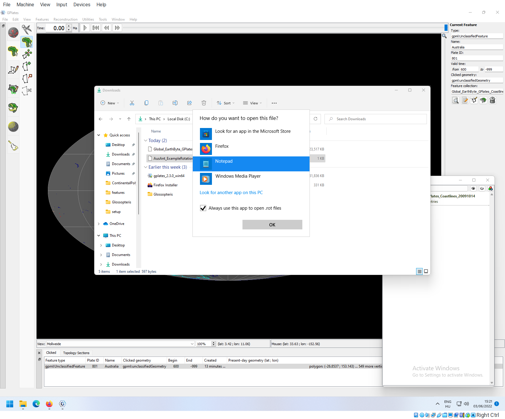
In the dialog box, that appears, select More apps,

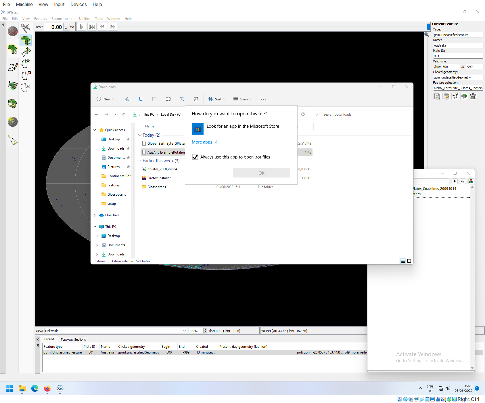
and then Notepad

The structure of the rotation file

The rotation file s a “whitespace-delimited” file, it has a table-like structure.

The headers are not included in the actual file, but here they are for convenience:

Plate ID	Age	Rel. Plate ID	Comment
001	0.0	000	!AHS-HOT Present day …
001	600.0	000	!AHS-HOT
701	0.0	001	!AFR-AHS Africa-Indian/Atlantic
701	600.0	001	!AFR-AHS
801	0.0	802	!AUS-ANT Australia-Antarctica
801	600.0	802	!AUS-ANT
802	0.0	701	!ANT-AFR Antarctica-Africa
802	600.0	701	!ANT-AFR
850	0.0	801	!TSM-AUS Tasmania-Australia
850	600.0	801	!TSM-AUS

Every row in this table describes the relative position of two entities (plates), that are identified by their plate IDs (Plate ID and Rel. Plate ID). Note that this structure means that the position of plate

001 relative to 000 (Indian/Atlantic hotspots relative to rotational axis)
701 relative to 001 (Africa relative to Indian/Atlantic hotspots)
802 relative to 701 (Antarctica relative to Africa)
801 relative to 802 (Australia relative to Antarctica)
850 relative to 801 (Tansania relative to Australia)

The relative positions are given as movements on the surface of the sphere that are added to the positions that are given in the polygon features (i.e. the coastlines). These movements are rotations that are described as Angles around a rotation axis. The rotation axis is given by its pole (Euler pole) that has longitude and latitude. Accordingly the relative positions are expressed with three values: Latitude, Longitude and Angle.

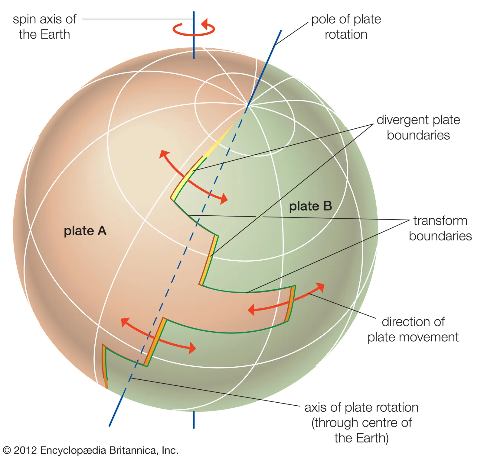
(0° 0° 0°) means that the relative positions of the plates are exactly the same as what they were in the the loaded spatial data, there is no movement.

Loading rotation files

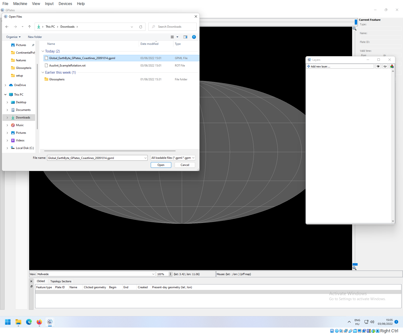
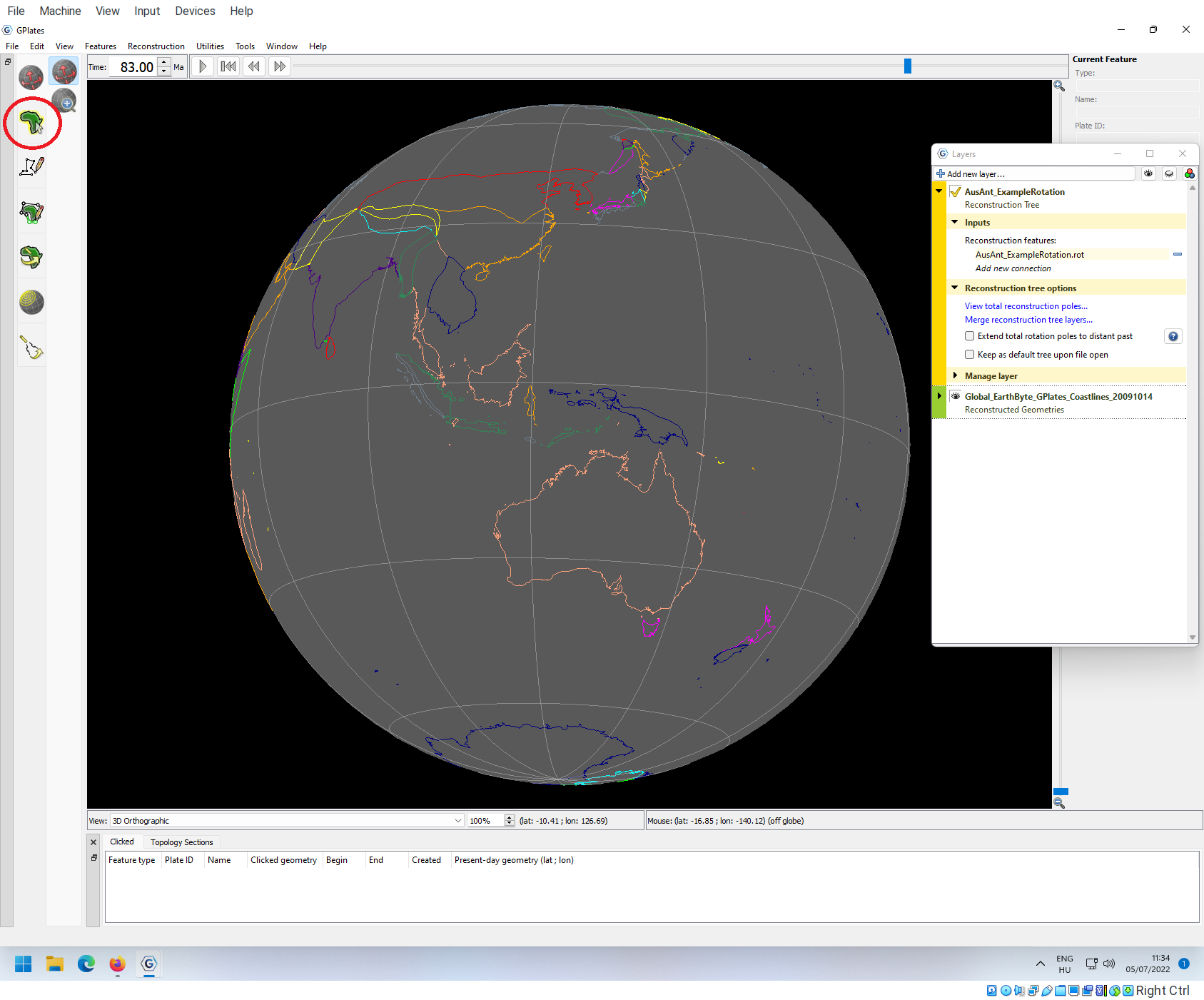
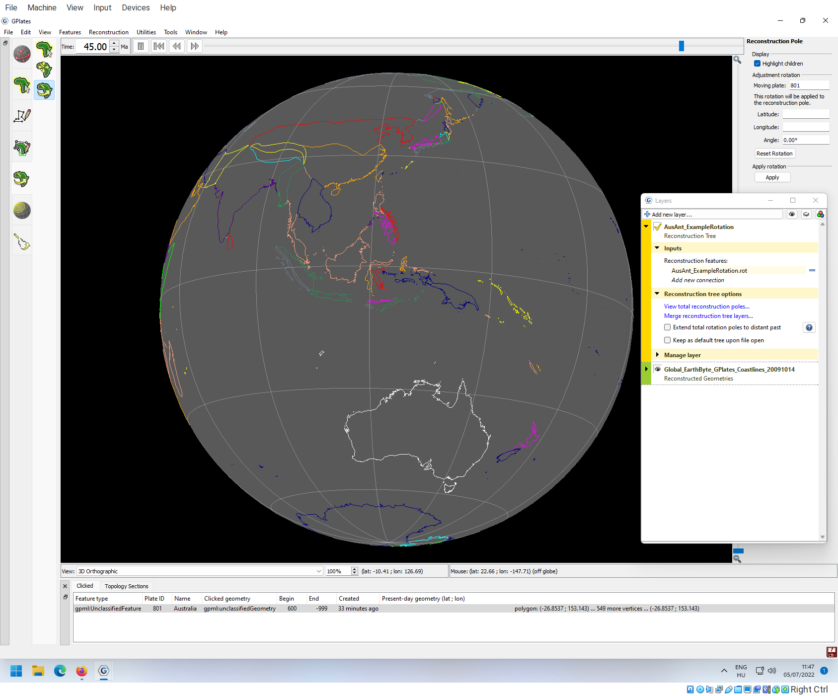
You can load in rotation files the same way as you would load other object, with the Open Feature Collection tool. Use this to load the AusAnt_ExampleRotation.rot along with the simplified coastlines Global_EarthByte_GPlates_Coastlines_20091014.gpml!

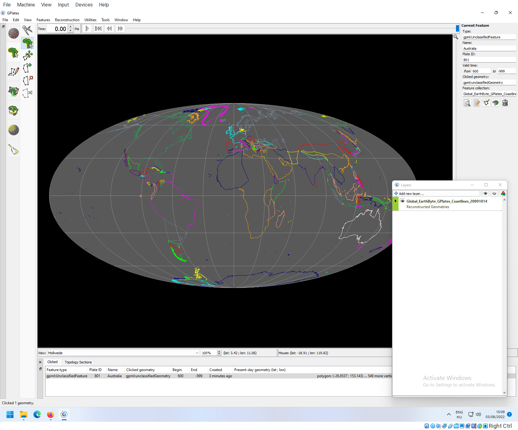
Once they are loaded you should see something like this:

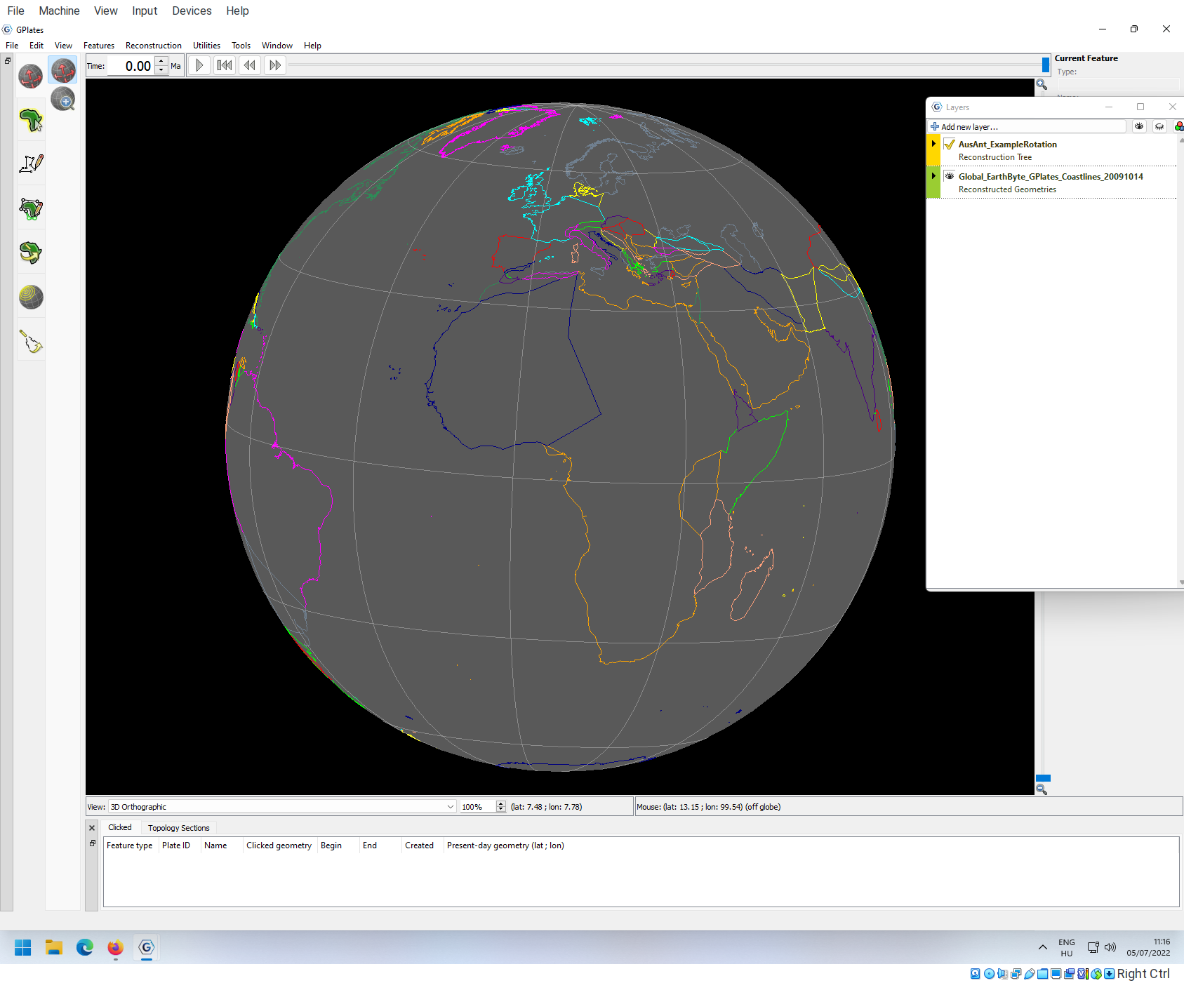
Note that the AusAnt_ExampleRotation layer in the Layer panel is yellow, indicating that this is a Reconstruction Tree object. If you move the time slider at the top some features disappear as we move out of their duration, but nothing will move yet.

This is because there are no actual rotations are implemented in the reconstruction tree.

Viewing the reconstruction tree in GPlates

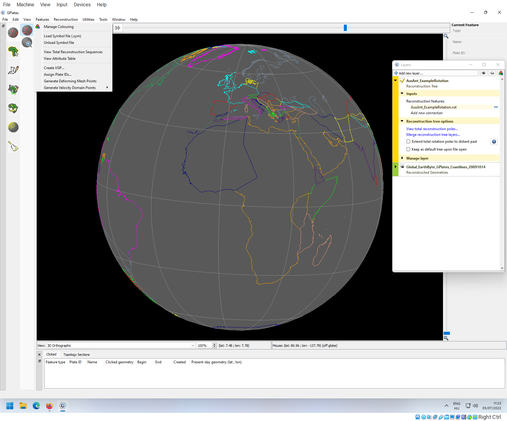
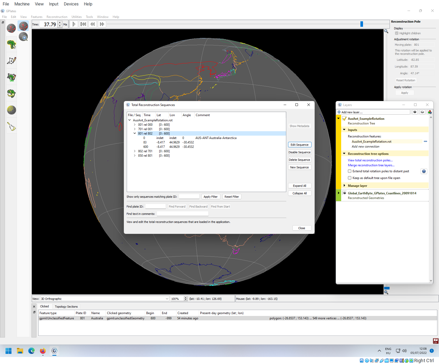
You can examine the loaded rotation file (Reconstruction Tree) if you got to Features->View Total Reconstruction Sequences.

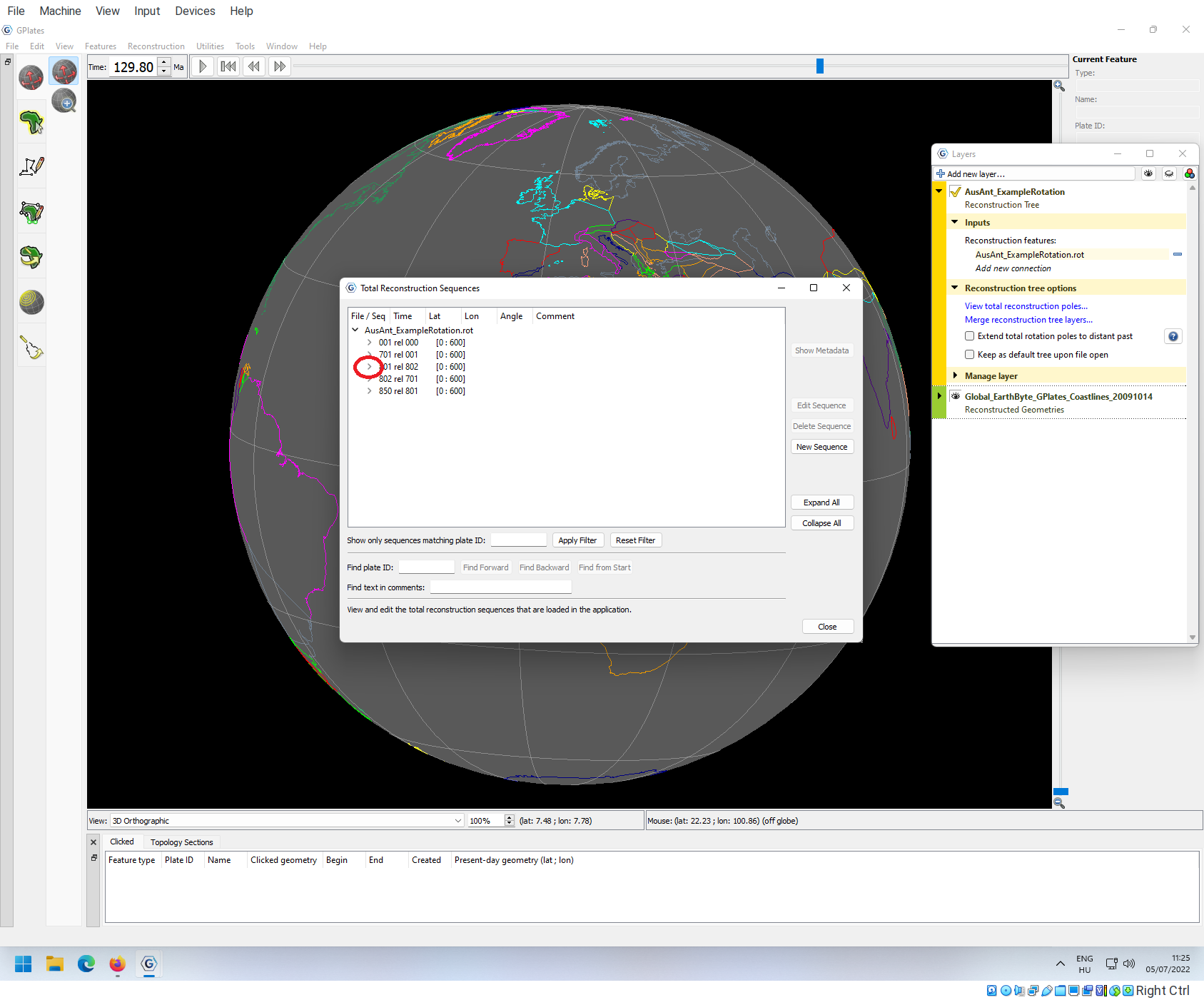
Here you can see the structure of the tree if you click on the little brackets before the rows

This information is the same as what you see in the loaded file if you open it in a text editor.

Implementing one rotation

The easiest way to understand what an actual rotation is, is to implement it ourselves. We are going to implement the northward drift of Australia (and Tansania) that started to split off from Antarctica about 83 million years ago.

To start, first set the time to 83Ma:

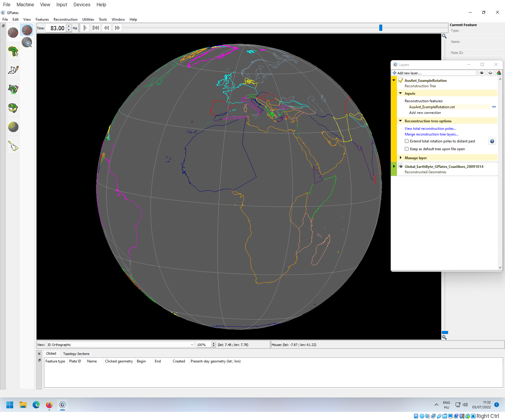
Choose a viewpoint where you can clearly see Australia and Antarctica.

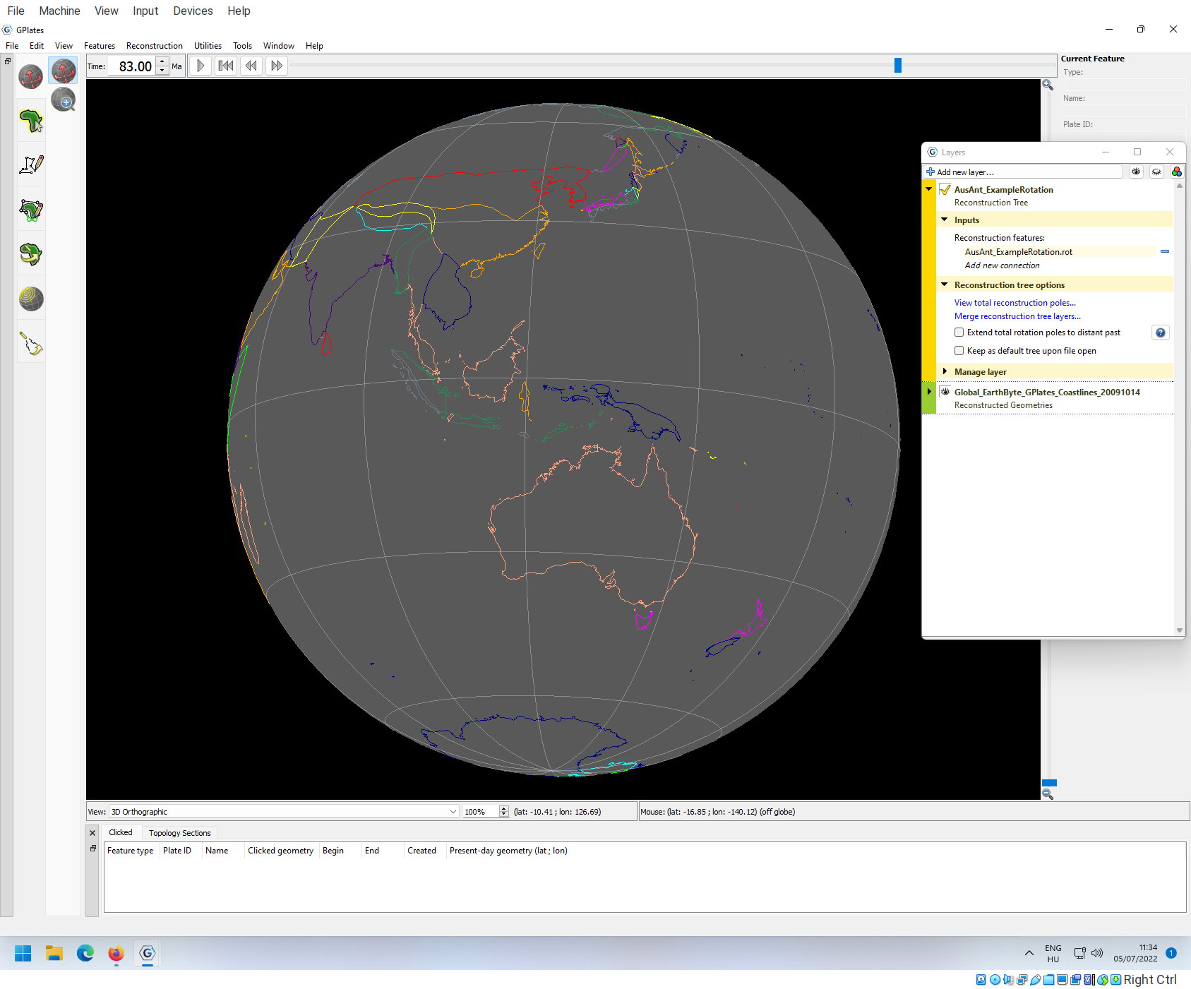
Use the Select features tool to select Australia.

To implement a rotation, use the Modify Reconstruction Pole tool, and drag Australia to the south, just so it touches Antarctica (you don’t need to be super precise here).

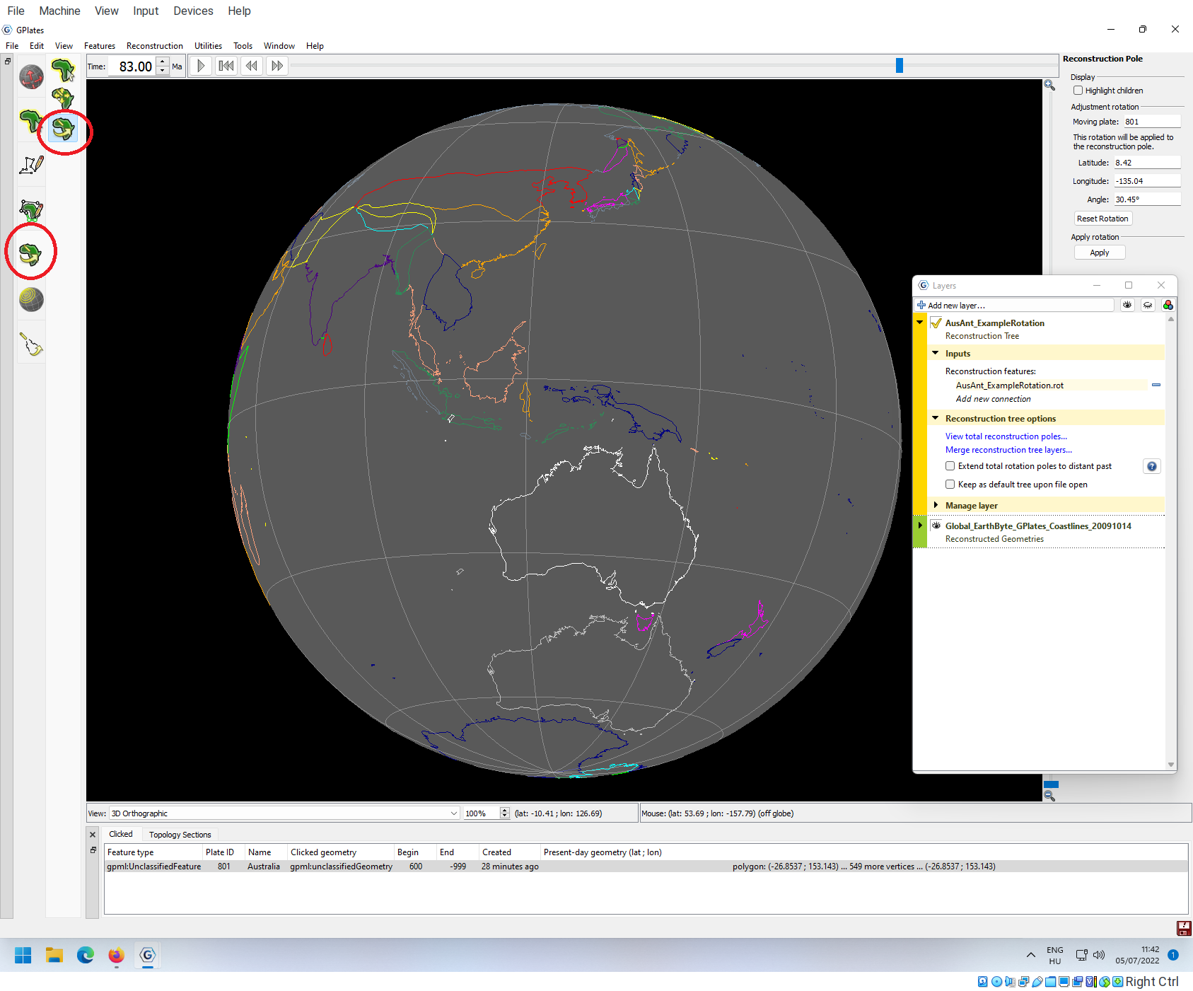
On the right-hand side you can see how the dragging changes the data of the rotation that you are implementing. The panel tells you what plate you are moving (801, Australia), the Euler pole of the rotation (latitude and longitude) as well as the angle of the rotation. There is a box that says Highlight children. Toggling this will show you how this single rotation might have effects on other plates that have positions that are relative to the position of Australia. If check this box, you will see the new position of Tansania.

You can always click on the Reset Rotation button to revert what you have done. But it you are fine with what you see, you can click Apply. When you do that, a new window will appear, summarizing all the changes that you are about to save.

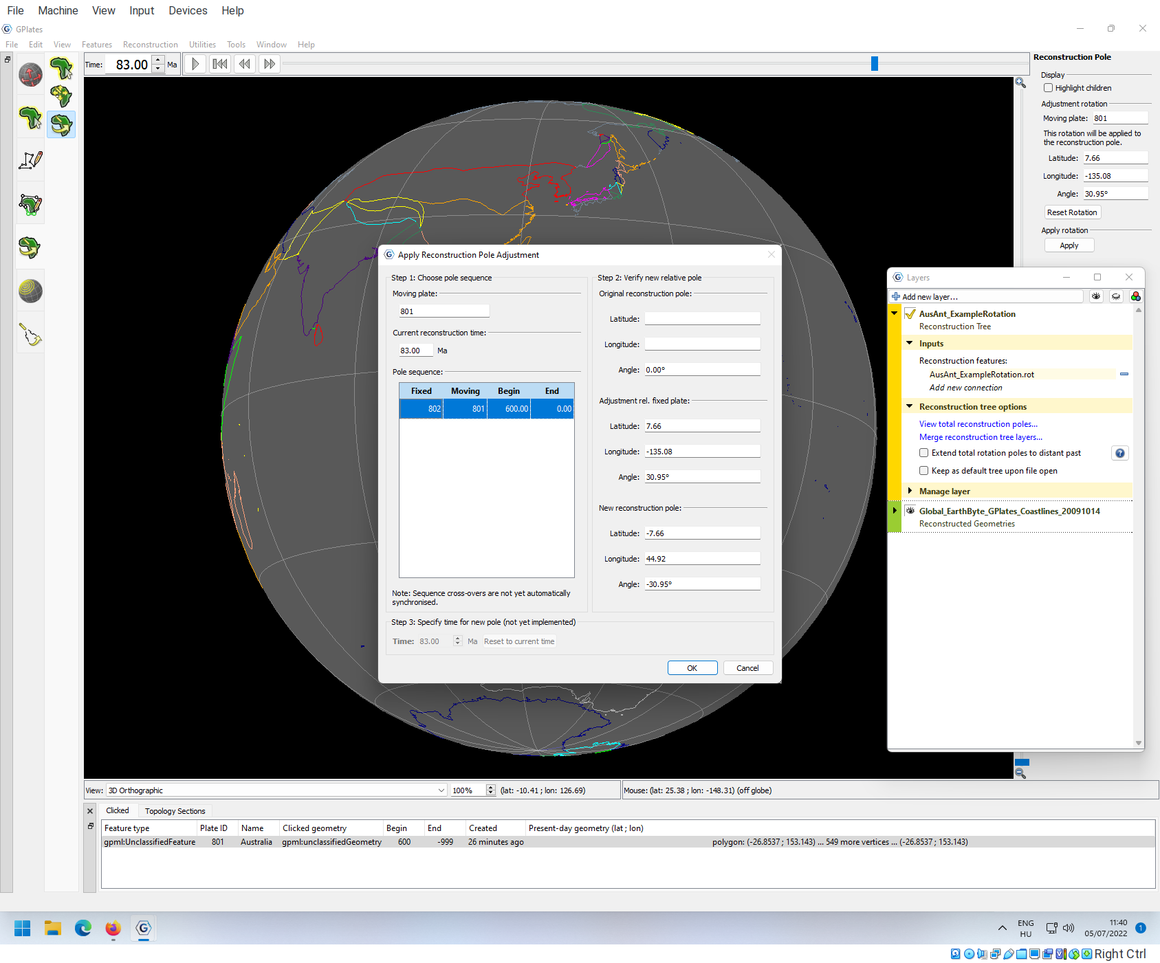
You can click Ok to see the changes.

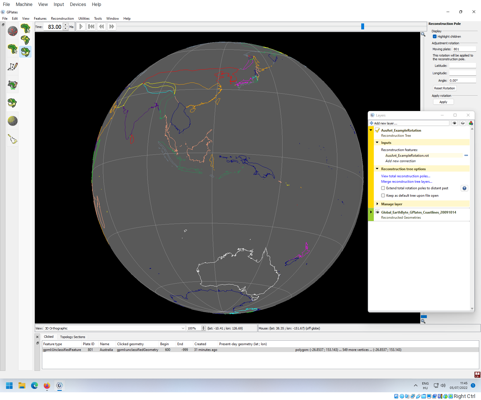
Congratulations for implementing your first rotation. If you click on the play button next to the age indicator, you will see Australia drifting northwards, until it reaches its present-day position at 0Ma.

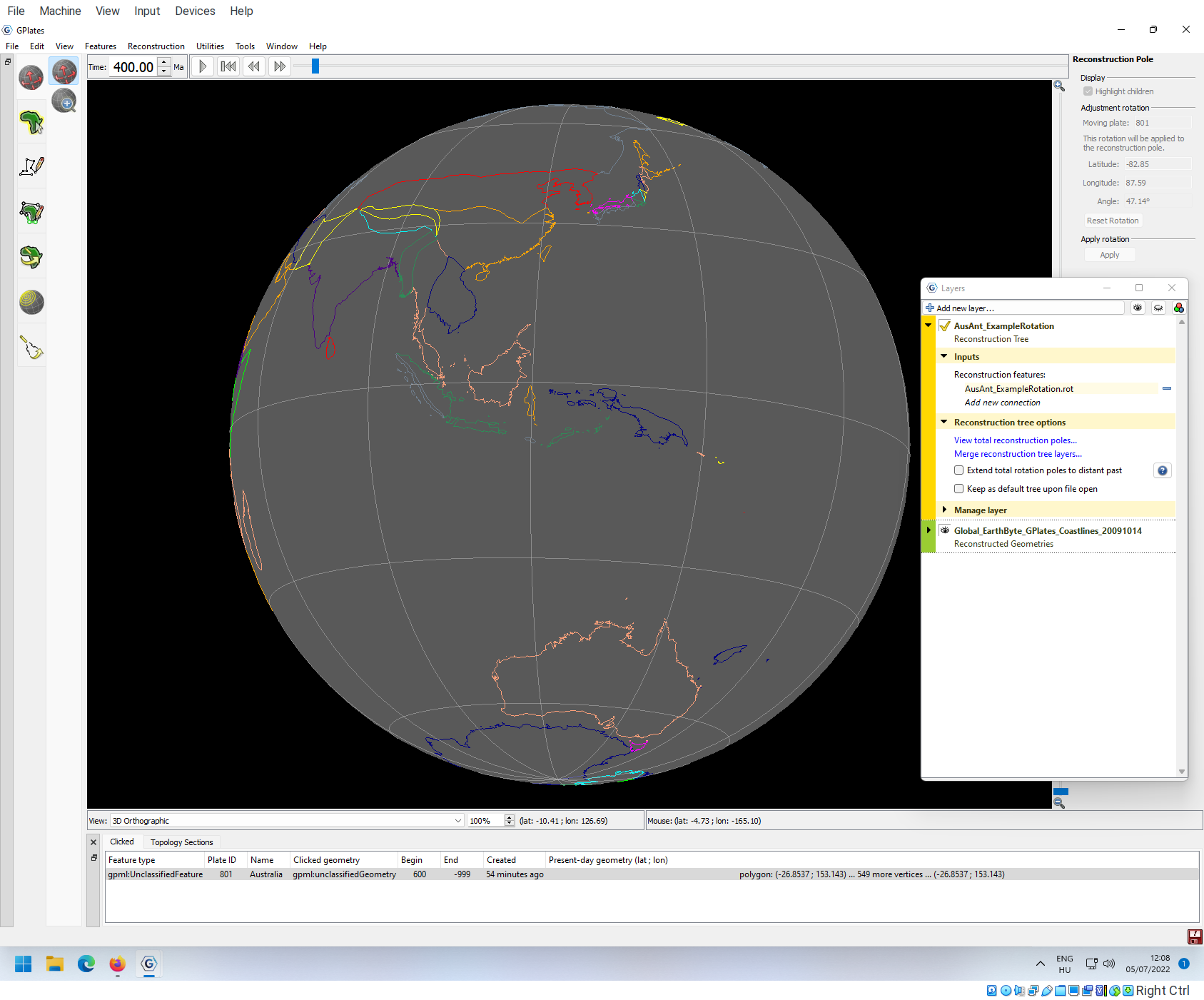
There is just one slight problem here… If you go back to say 400Ma and start the animation from then, you will see that Australia is again to the north from Antarctica, slowly drifting to the south.

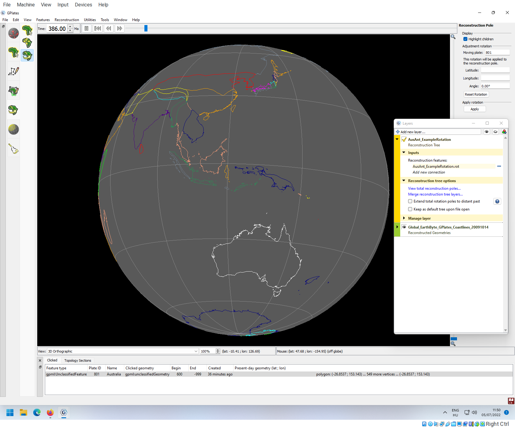
This southward drifting goes on until Australia reaches its southermost position in the model, at exactly 83 Ma. Let’s check out the reconstruction tree, what we actually have. Go to Features-> View Total Reconstruction Sequence and unfold the entries until we see all information for plate Australia (801 relative to 802).

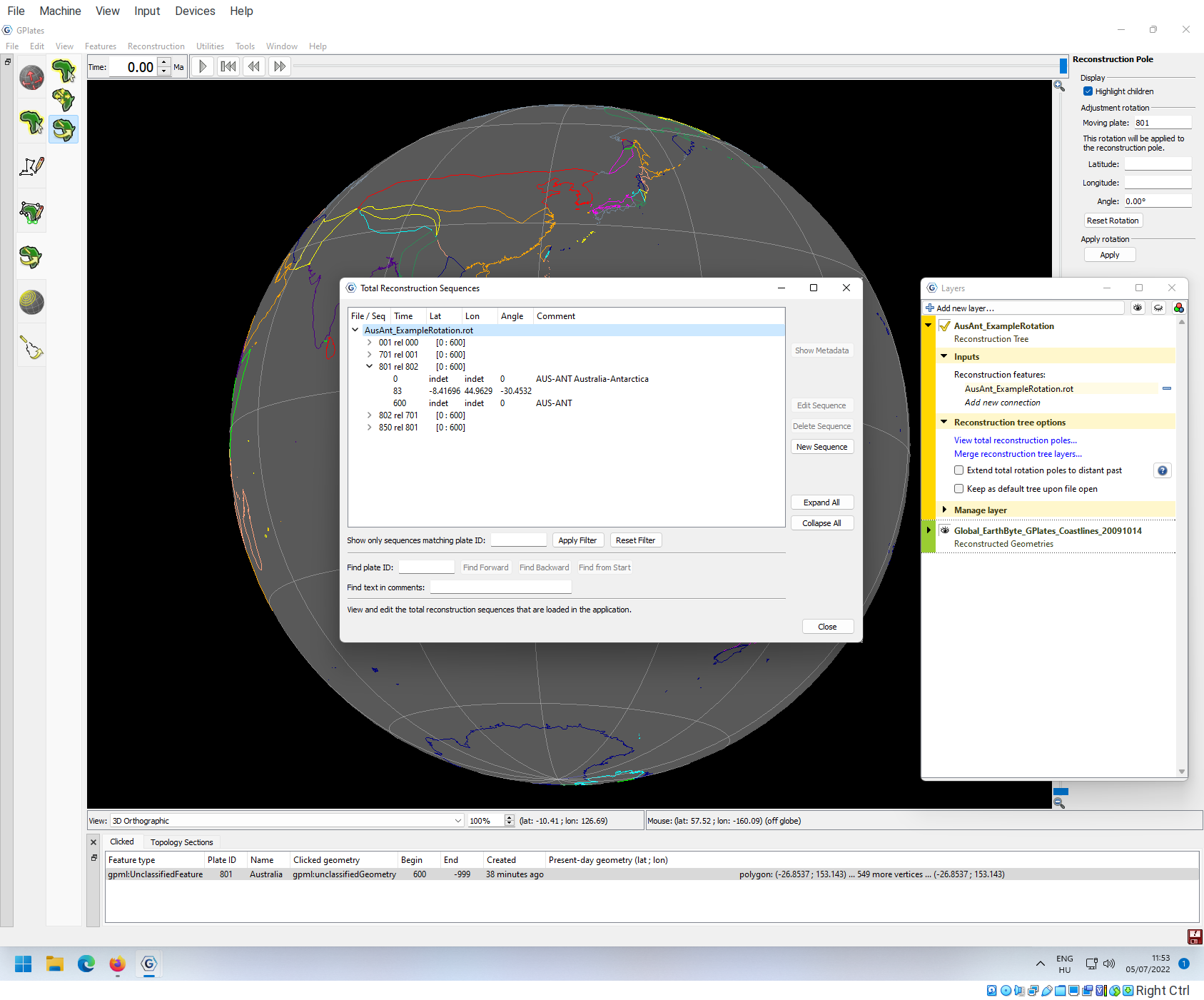
What is defined in these three rows is that 600 Ma, Australia is at its present-day position relative to Antarctica, gets into the rotated position by 83 Ma, and then it goes back to the present-day position. We don’t need the last row, so we need to edit this bit. Click on the row of 801 rel 802 and click on Edit Sequence.

A new window will pop up, where you can edit graphically what you saw in the previous window.

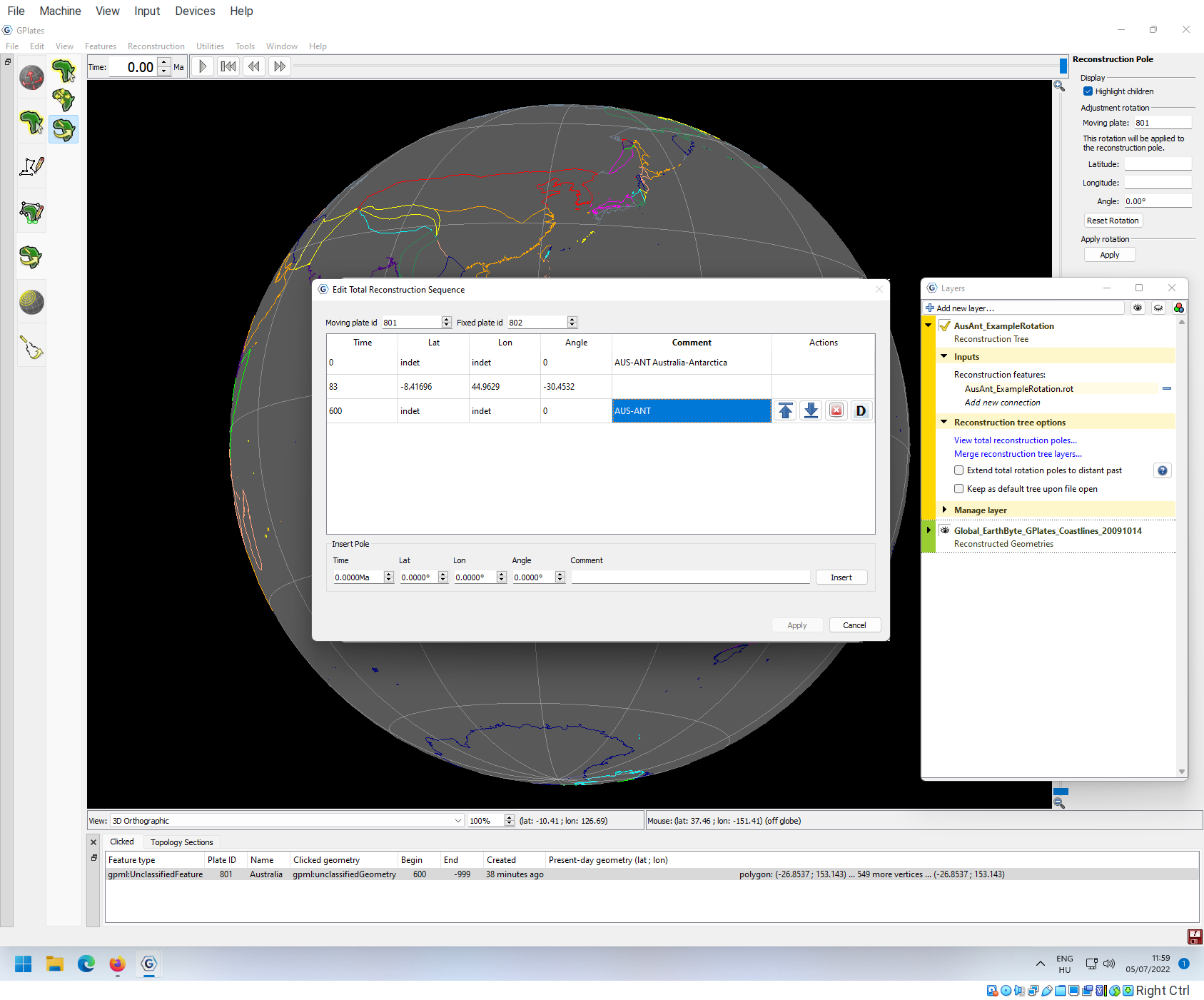
We want to make the position of Plate 801, to be the same at 600 Ma as what it was at 83Ma. For this, we have to copy over the Lat, Lon and Angle values from the second row to the third.

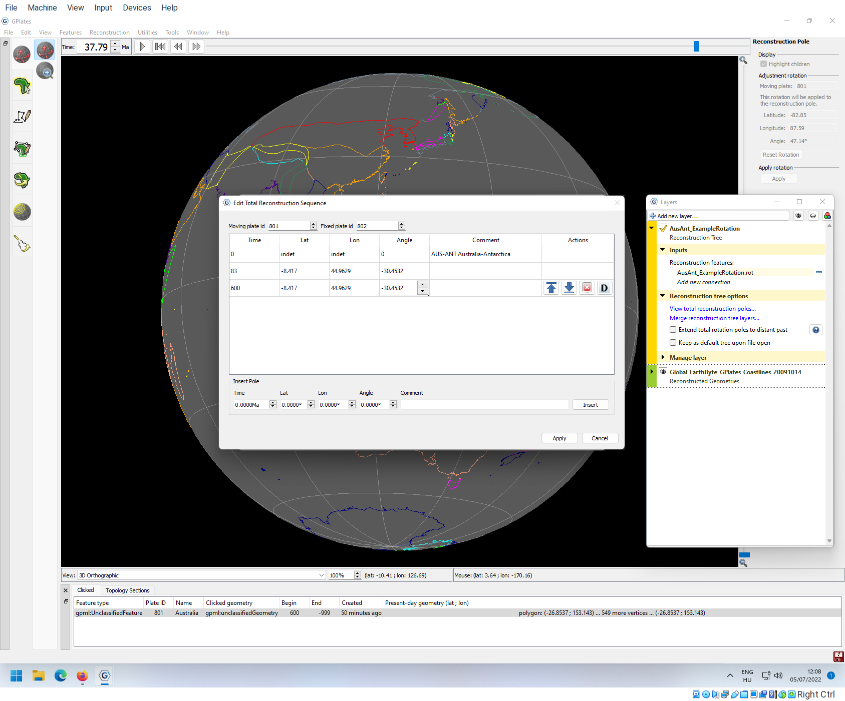
Clicking on Apply at the bottom will save these changes. Then you need to get out of the window by either hitting Cancel. Note that your changes have been processed:

Then you can click on Close.

If you go back to 400Ma, you will see that Australia is still at its southern position, connected with Antarctica.

Saving changes

Note that if you go to the File -> Manage Feature Collections menu item, the rotation file is now red, indicating that the loaded object is not what is in the file:

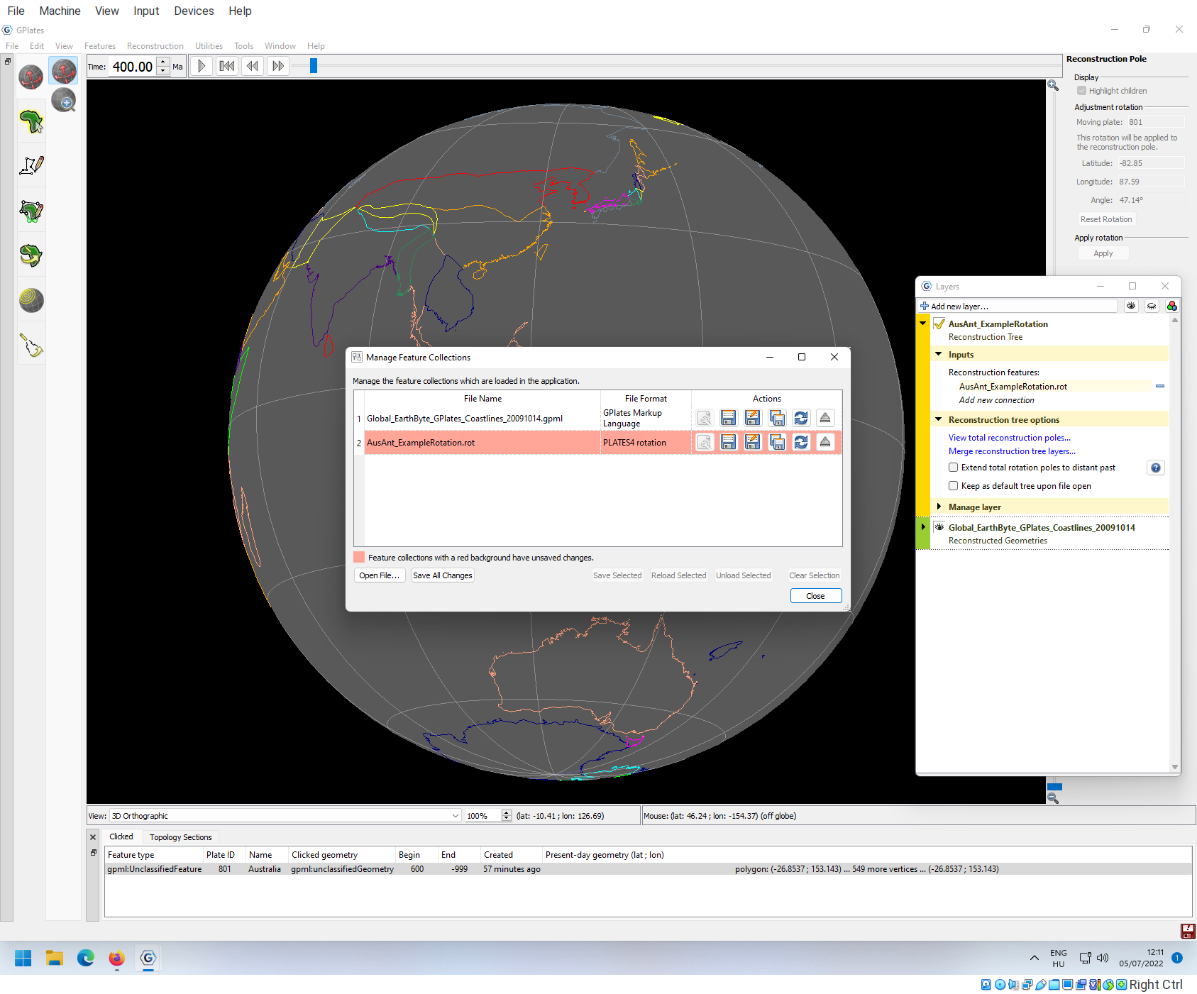
Note that if you do not save your changes here, then they would not be saved to the hard drive!

Entire reconstructions

Now a single rotation is finished. A complete plate tectonic reconstruction consists of thousands of such simple rotations, which takes years to develop - which is why we want to rely on published rotation models for doing any kind of paleogeographic reconstruction.