Basic features
- Loading feature collections
- Inspecting features
- Loading a second set of features
- The Layers window
- Exporting Snapshots
- Unloading features
GPlates comes with a lot of example data that helps you better understand how the program works. These data can be loaded as feature collections.
Loading feature collections
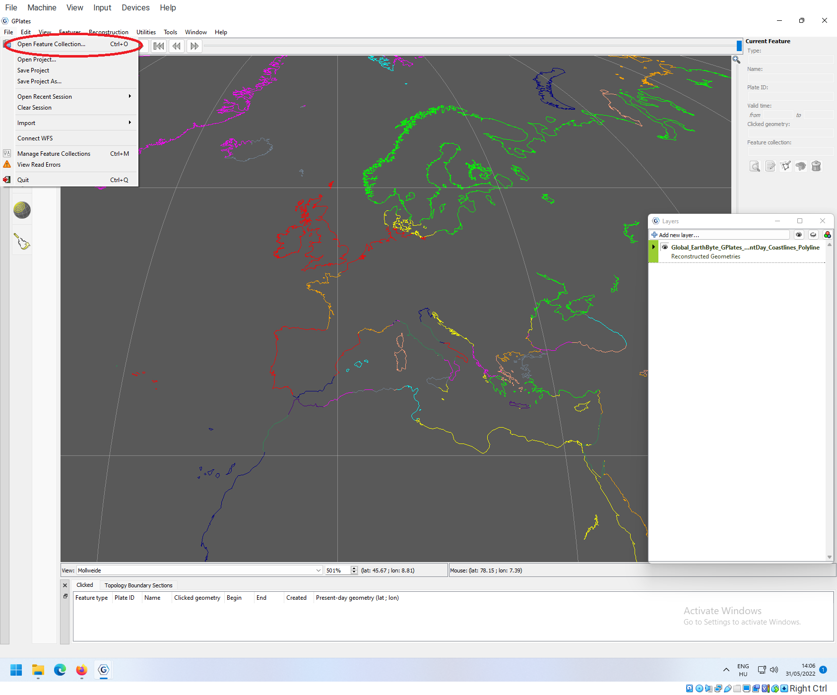
New feature collections can be loaded by Clicking File->Open Feature Collection….
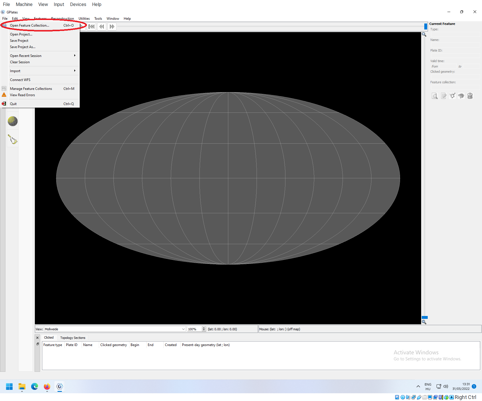
This will open up a dialogue window that lets you select files to load. By default it will open up in a directory, where example data are located.
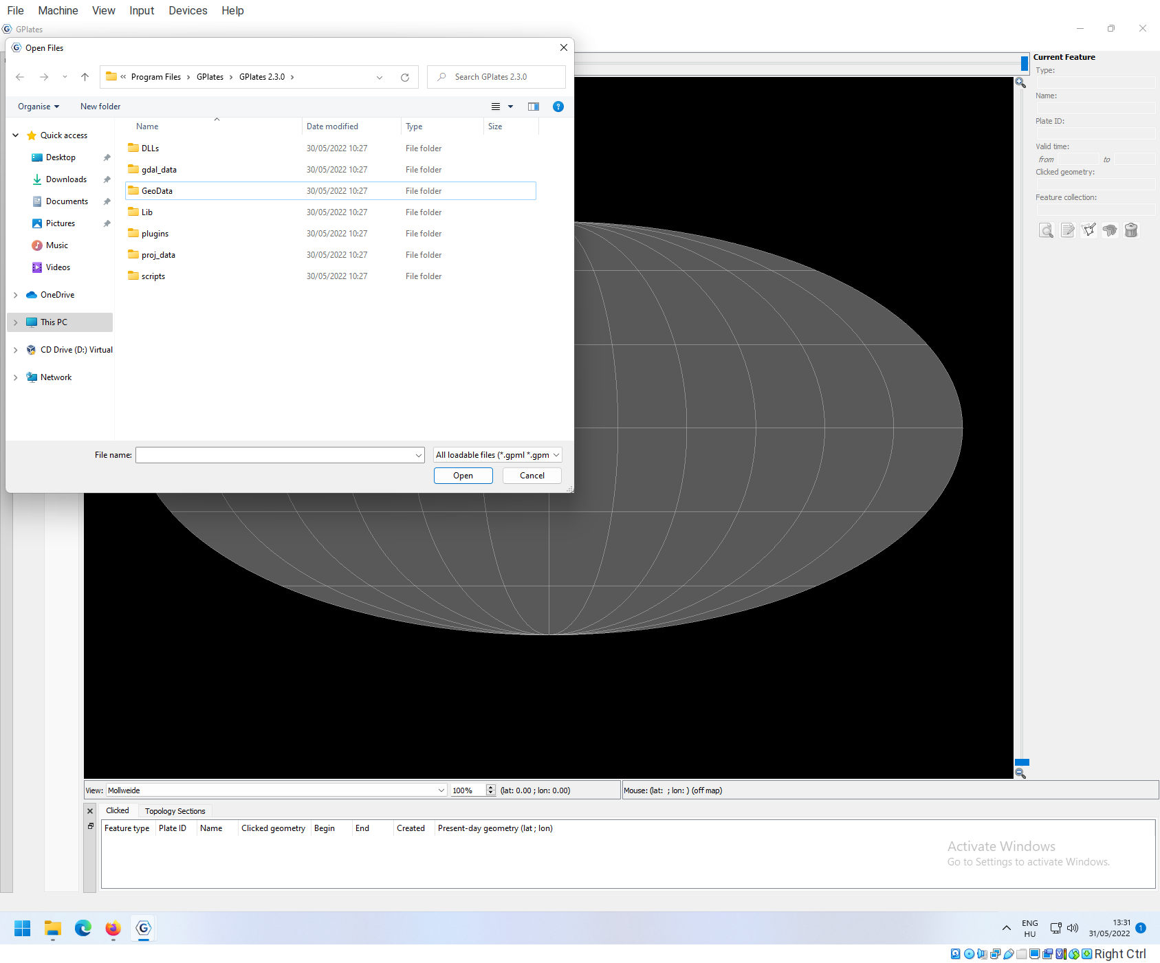
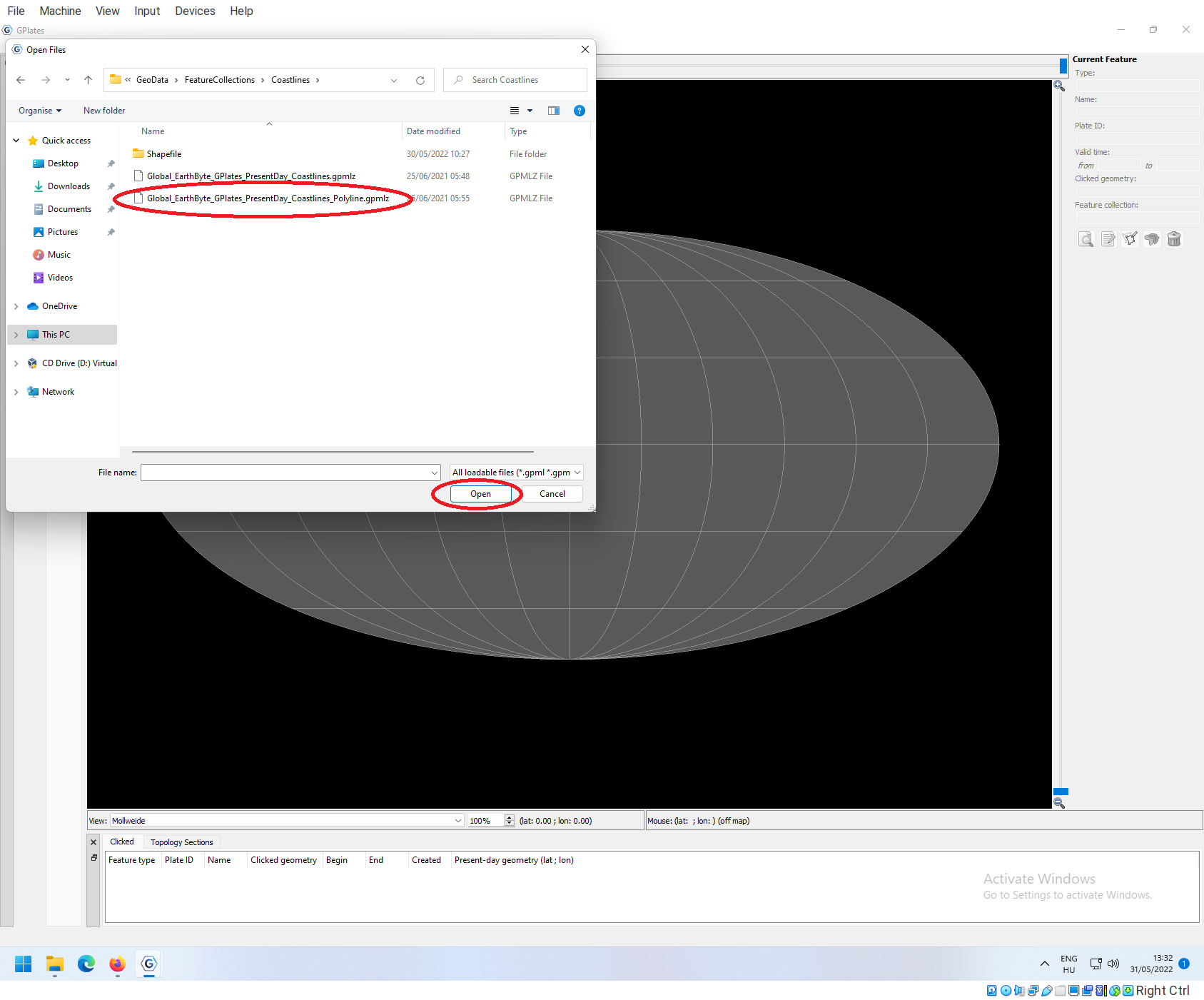
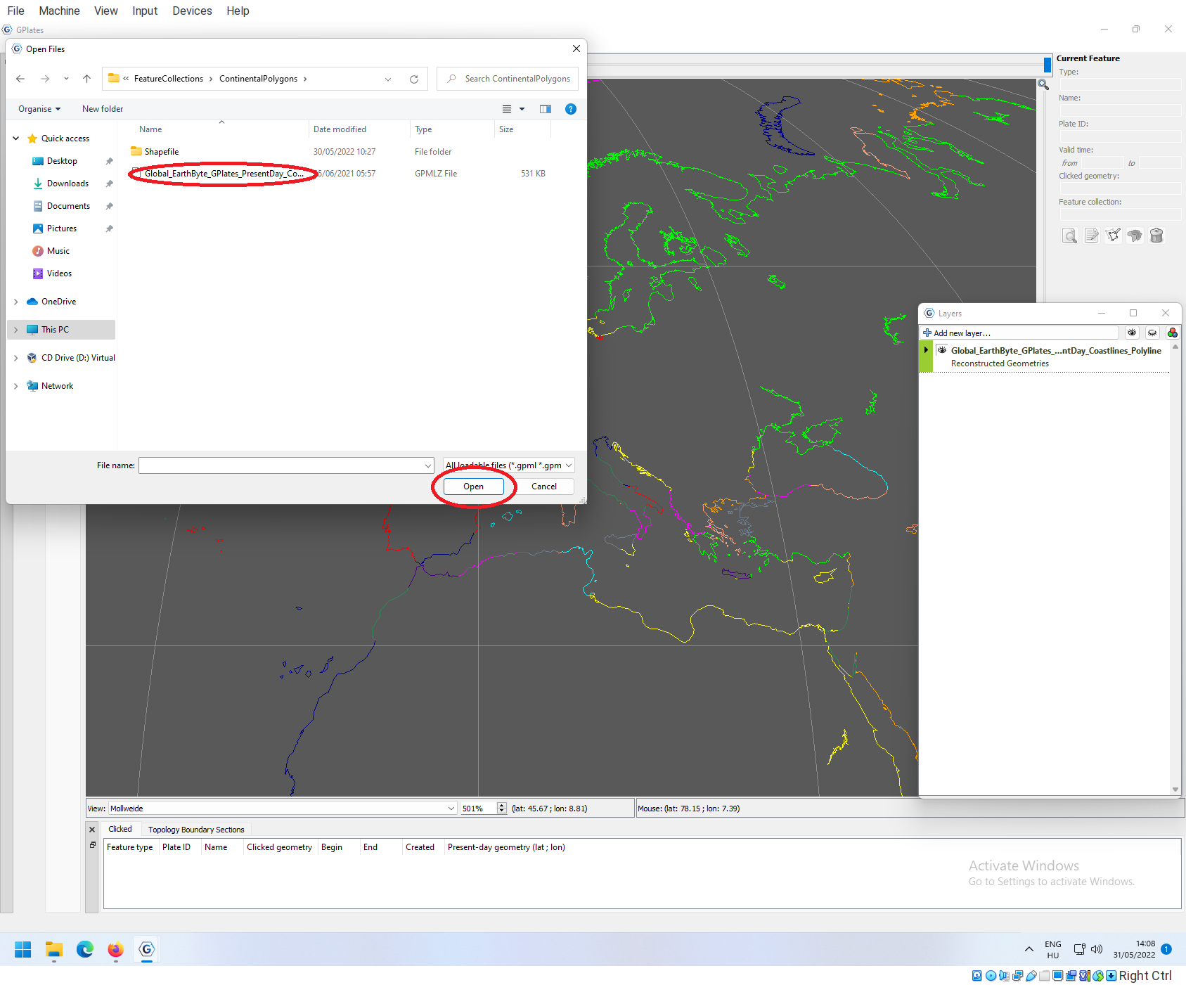
Note that there is a folder called GeoData, which includes all the example data that comes bundled with GPLates. Let’s load a feature collection! In this dialogue window navigate to GeoData/FeatureCollections/Coastlines. You should see the following files
Note in the bottom right corner the extension that the file opening explorer window is searching for: all loadable files(*.gpml etc.). These are all the different GPlates-native file formats. If you see *.proj here, that means that you have clicked on Open Project instead. Projects are current states of the GPlates application, with which you can continue working from where you have left off, wheras Feature collections are the individual data that you can import into the program.
You open a Feature collection by double clcking on it. Let’s open Global_EarthByte_GPlates_PresentDay_Coastlines_Polyline.gpmlz!
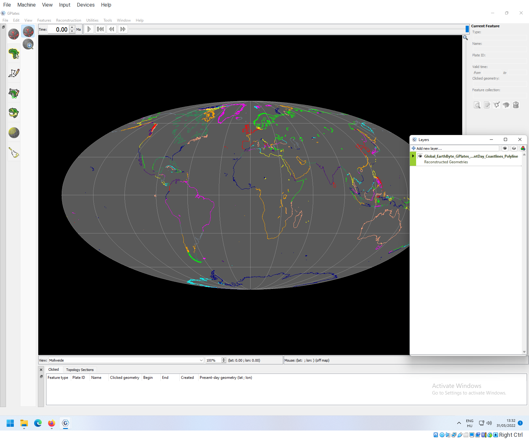
Loading the feature collection will inflict two changes: 1. You will see a map appearing in the reconstruction view, and 2. the Layers window will pop up. Note that the projection in set to Mollweide!
Inspecting features
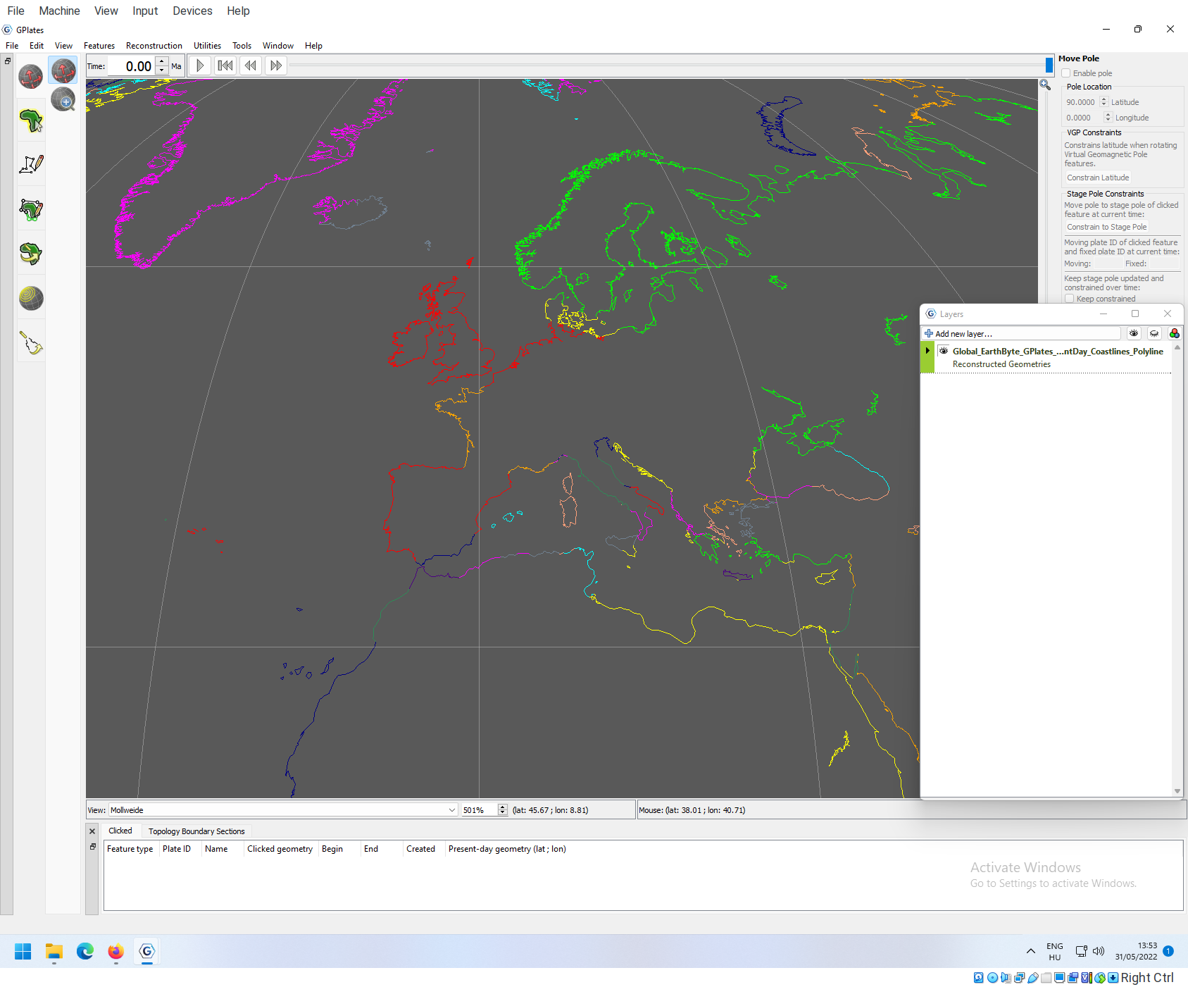
The loaded map displays coastline segments with different colors, which is even more apparent, when you zoom into the map.
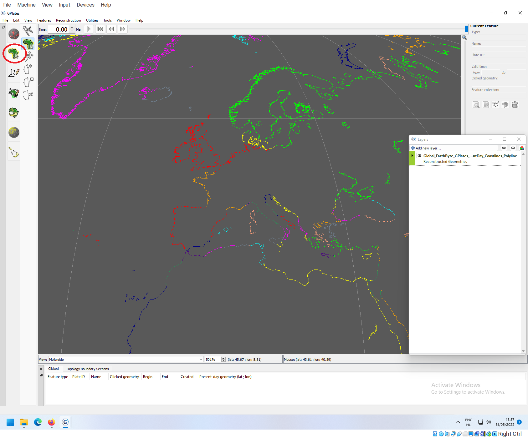
You can use the Inspect features tool to find out more about these individual segments. This tool is the second symbol in the tools at the right hand side.
Then you can click on the individual segments to select them. Note that the selected segment will turn white. In this case this is the Atlantic coast of the Iberian peninsula.
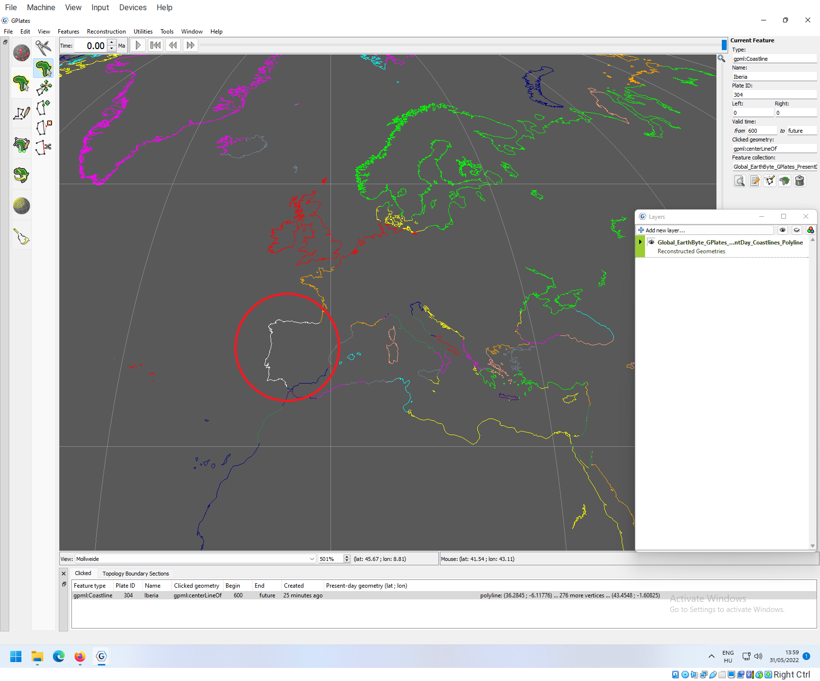
When you click on a feature, the right-hand panel under Current feature will display details of the currently active feature. Among many attributes, features have Names, in this case this is “Iberia”. They also have a PlateID, which in this case is 304. But why are they colored? It will make more sense if we load in another feature.
Loading a second set of features
You can load in as many features as you want by going to File->Open Feature Collection…, as before.
It is likely that the dialogue window will pop up where you opened the previous file. Let’s go back to the FeatureCollections folder and go into ContientalPolygons from there.
Here open up the only file: Global_EarthByte_GPlates_PresentDay_ContinentalPolygons.gpmlz!
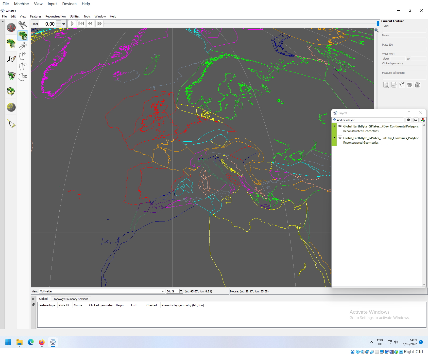
After loading, the map will change again, and a new entry will be added to the Layers window.
This second feature, iincludes outline polyongs of the continental plates. You can inspect them similarly as the coastline segments. Clicking on the outlines of the polygon surranding the main part of the Iberian peninsula (red), will highlight the entire polyong as white. Its name is also Iberia and its Plate ID is also 304.
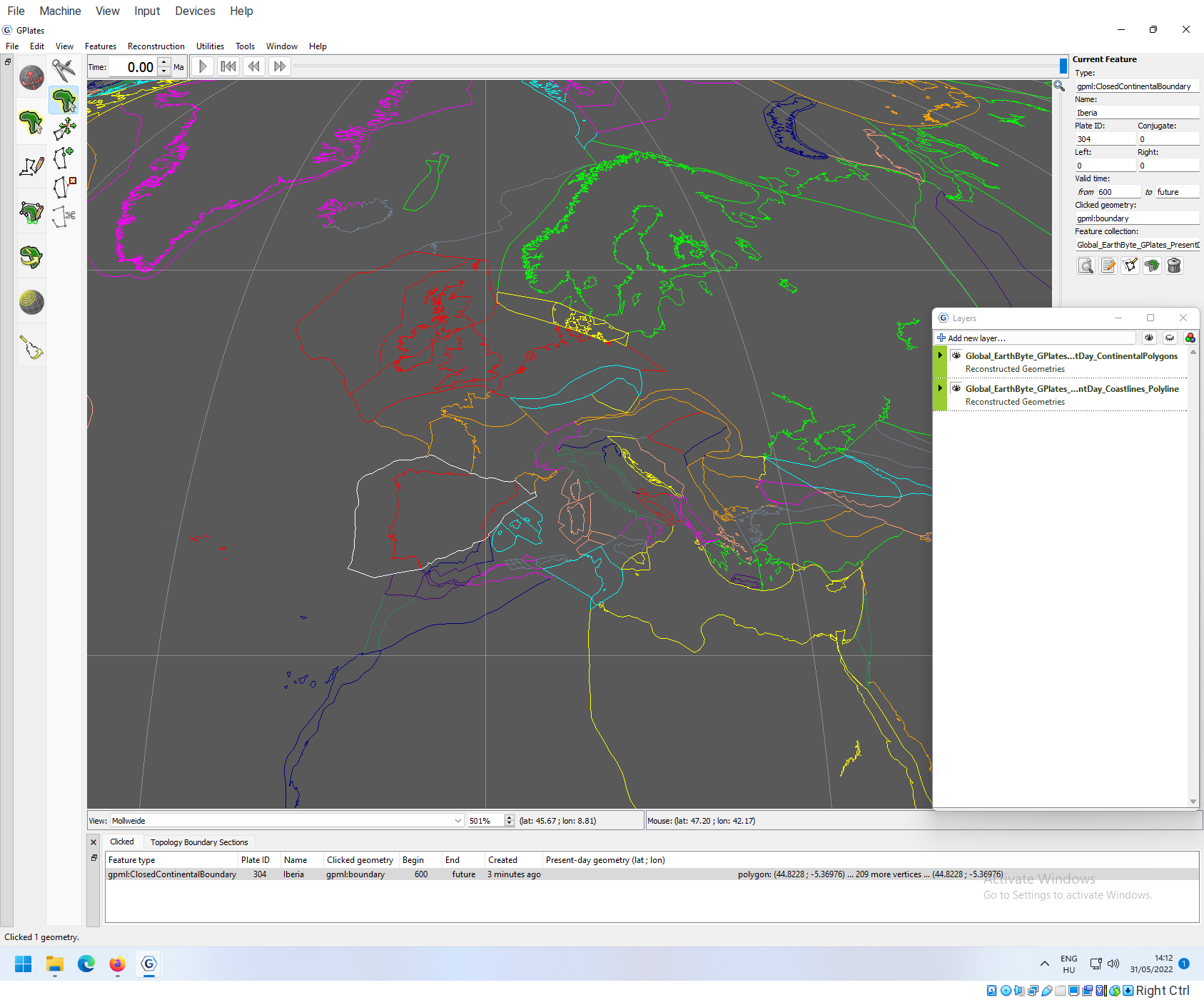
What you see is how the underlying continental polygons partition the present-day coastline. If you select any of the coastline segments, you will see that the surrounding polygons will also have the same colors, and they will have the same Plate ID. As a matter of fact, the colors are selected to indicate the Plate ID. These are very important: the movement of the plates are described by referring to their Plate IDs.
The Layers window
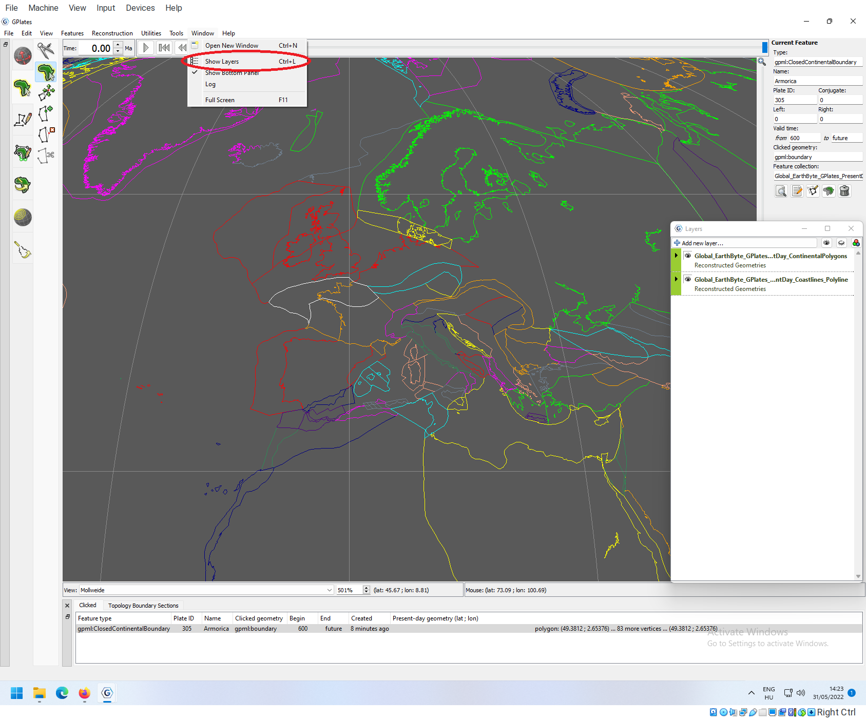
The layers window is used to organize feature collections and to tidy up your workspace. You can always turn the Layers window on and off by going to Window->Show Layers in the top menu, which can be handy in case you lose it.
Note that the window can also be minimized by clicking on the minimize bar in the top right corner of the window, and then the window will be minimized to the the taskbar of GPlates.
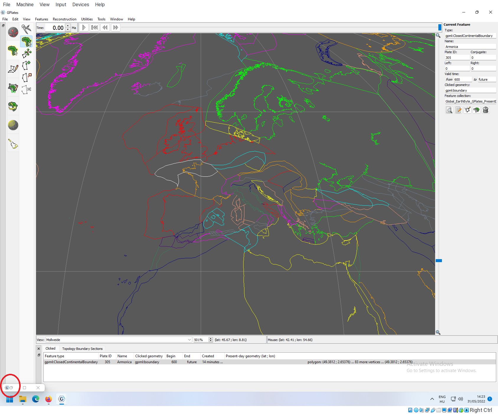
If you lose the Layers window, be sure to check it there! You can always expand this by clicking on the icon to restore the window.
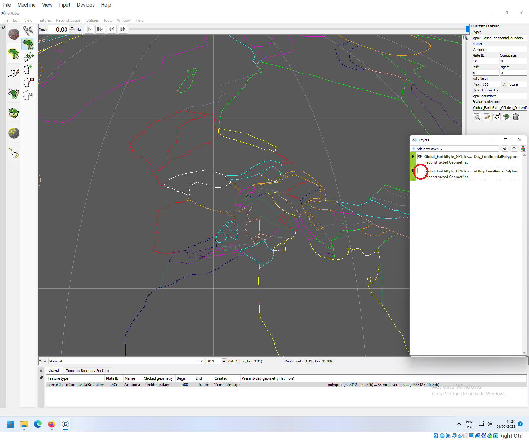
You can turn on the visibility of individual Feature collections (layers) by clicking on the little eyes. This is what the polygons themselves look like, if you turn the coastline polyine invisible:
You can also look at more details of the feature collections by clicking the little triangle at the left-hand side of the entry (left to the eye):
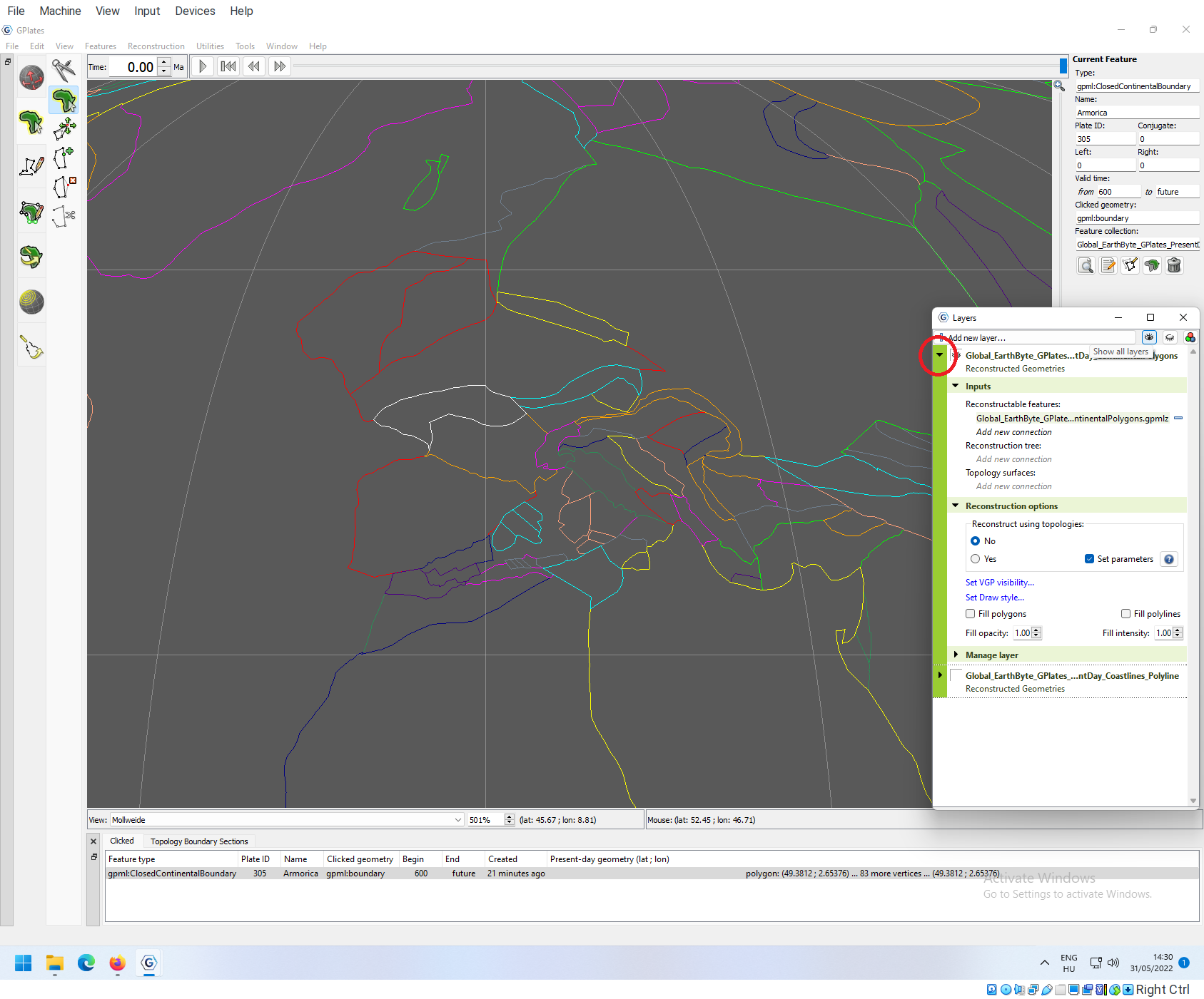
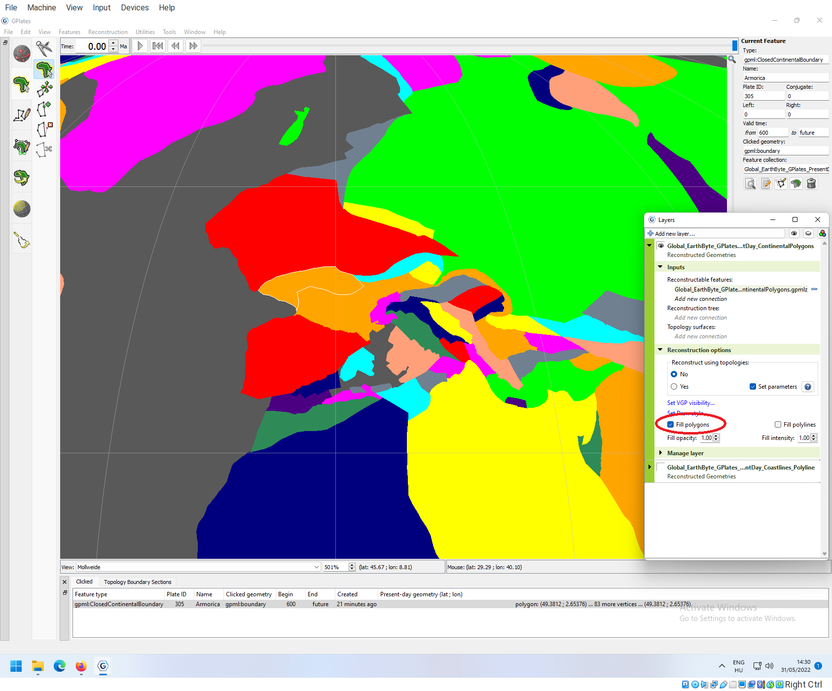
The Inputs field describe where information is coming from and how other feature collections influence the behavior of the current one. Reconstruction options allow you to select how the current reconstruction (e.g. visualization) is happening. For instance, the current features are polygons. You can fill them with their respecitve colors if you click on Fill polygons.
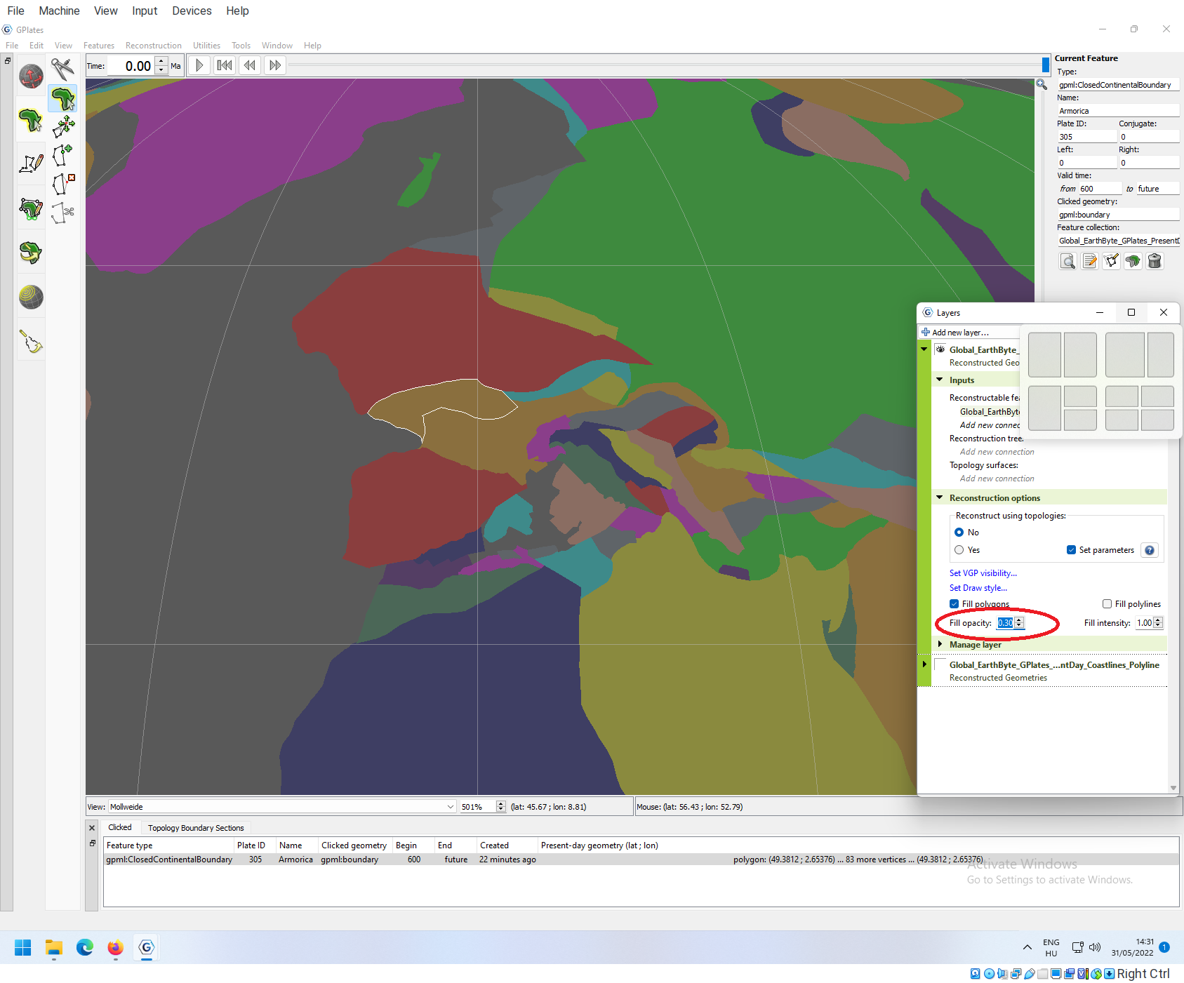
Now the plate structure becomes even more apparent. You can make the colors less obnoxious is you decrease the fill opacity (opposite of transparency) to a lower value, say 0.3.
If you want to you can always just add back the coastlines by clicking on the box where the little eye is, and then it will be clear how this particular plate tectonic model partitions the coastline to segments.

Exporting Snapshots
For those of us who do not work on making better models for reconstructions, the primary output of GPlates is going to be either some kind GIS data (later), or just simple images.
Both of these fall into the category of exporting. These can be done by going to Reconstruction->Export… in the top menu.
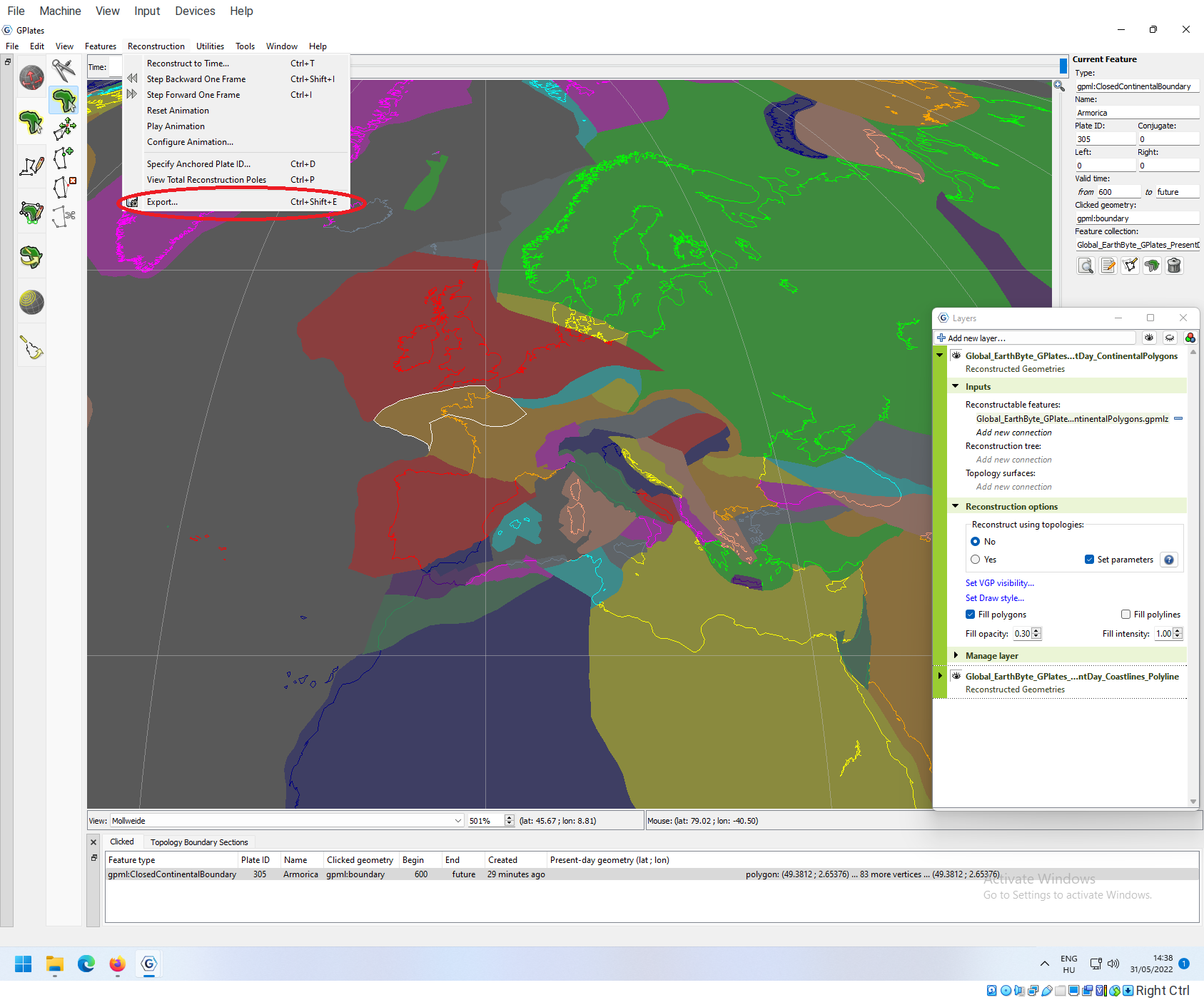
Clicking on this entry will open up the Export dialog window.
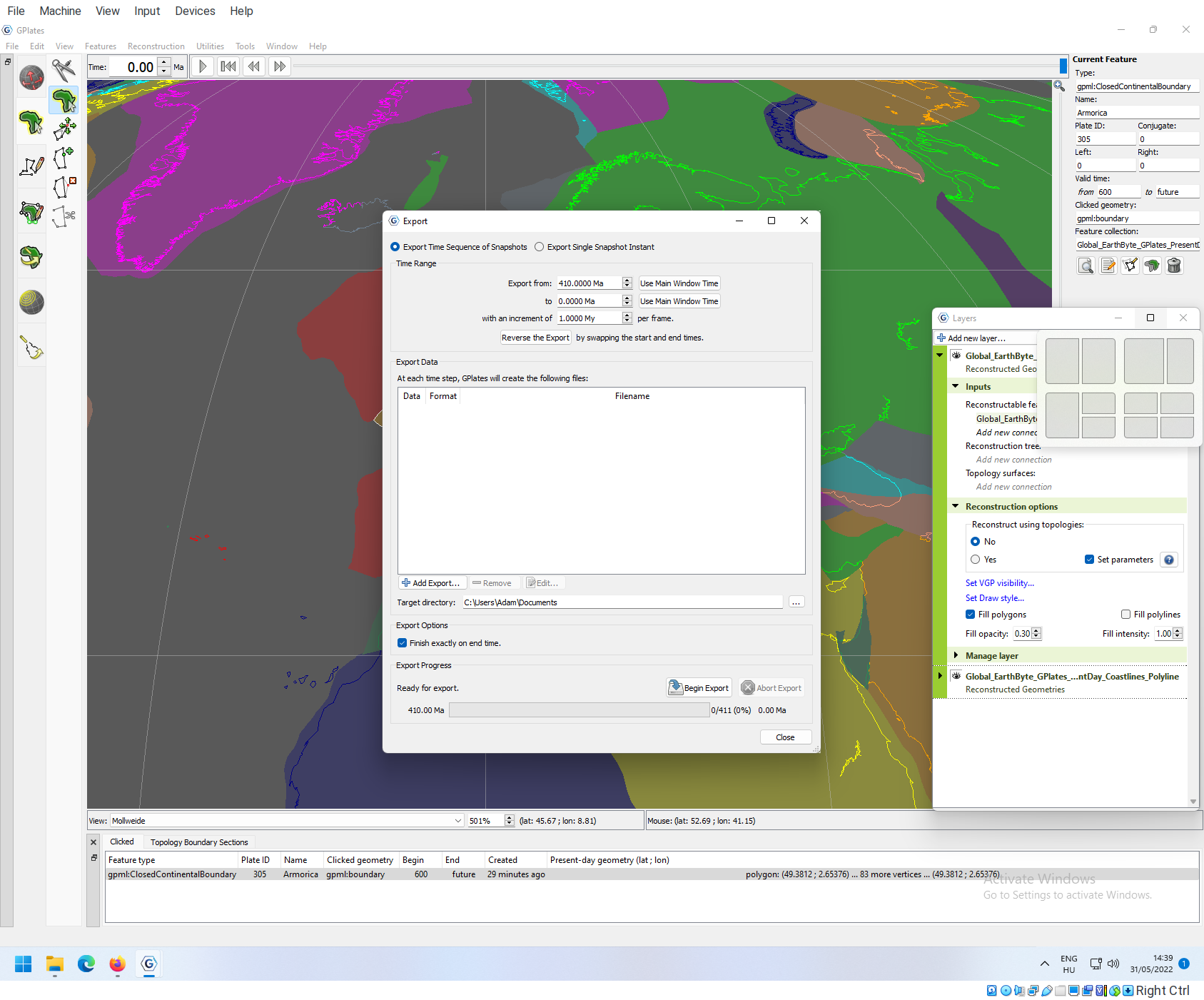
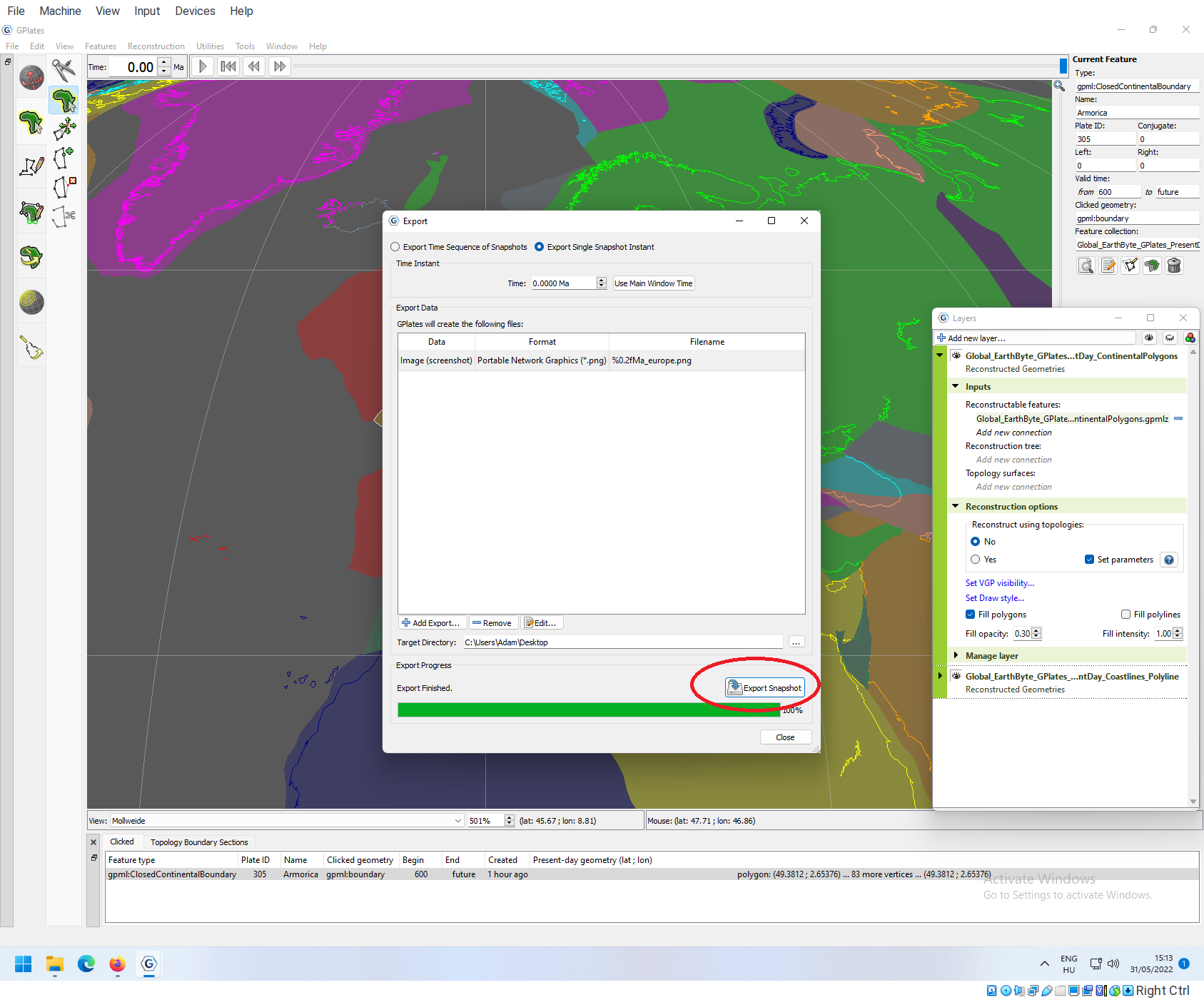
GPlates is used primarily to reconstruct information that changes over time. Accordingly you either want to export a sequence of states (either data or images, for instance to make animations with it), or just a single snapshot. Our current example (coastlines and continental polygons) conveys information about the present state of things, so for this example clicking Export Single Snapshot Instant at the top is more suitable.
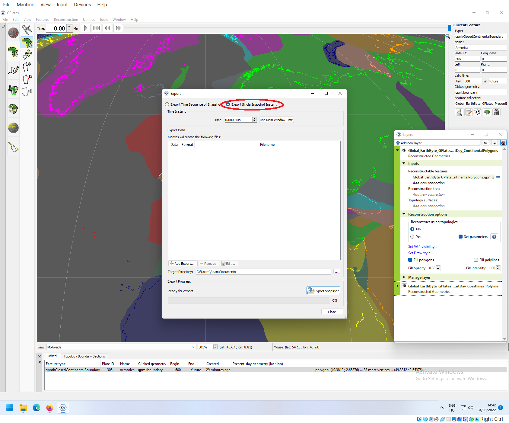
Note that the top rectangle was immediately simplified, we only need to concern ourselves about one moment in time. In this example this is set to 0.0000Ma that is the present-day. This is also the date that you see in the top-left corner of the main window.
The first thing that we need to specify is what and how we want to export. For this, we have to click on Add Export:

This will open up a new dialog window, with four steps:
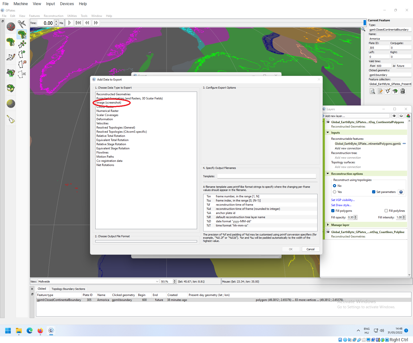
The first step is to choose the output data. You can see the range of options here. The two most frequently used ones are Reconstructed Geometries that are the GIS data of how the features are positioned at the time of the reconstruction, and Image (screenhots).
Let’s make a screenshot of the reconstruction view. After clicking on Image (screenshot), you can 2. select the type of image that you want to produce:
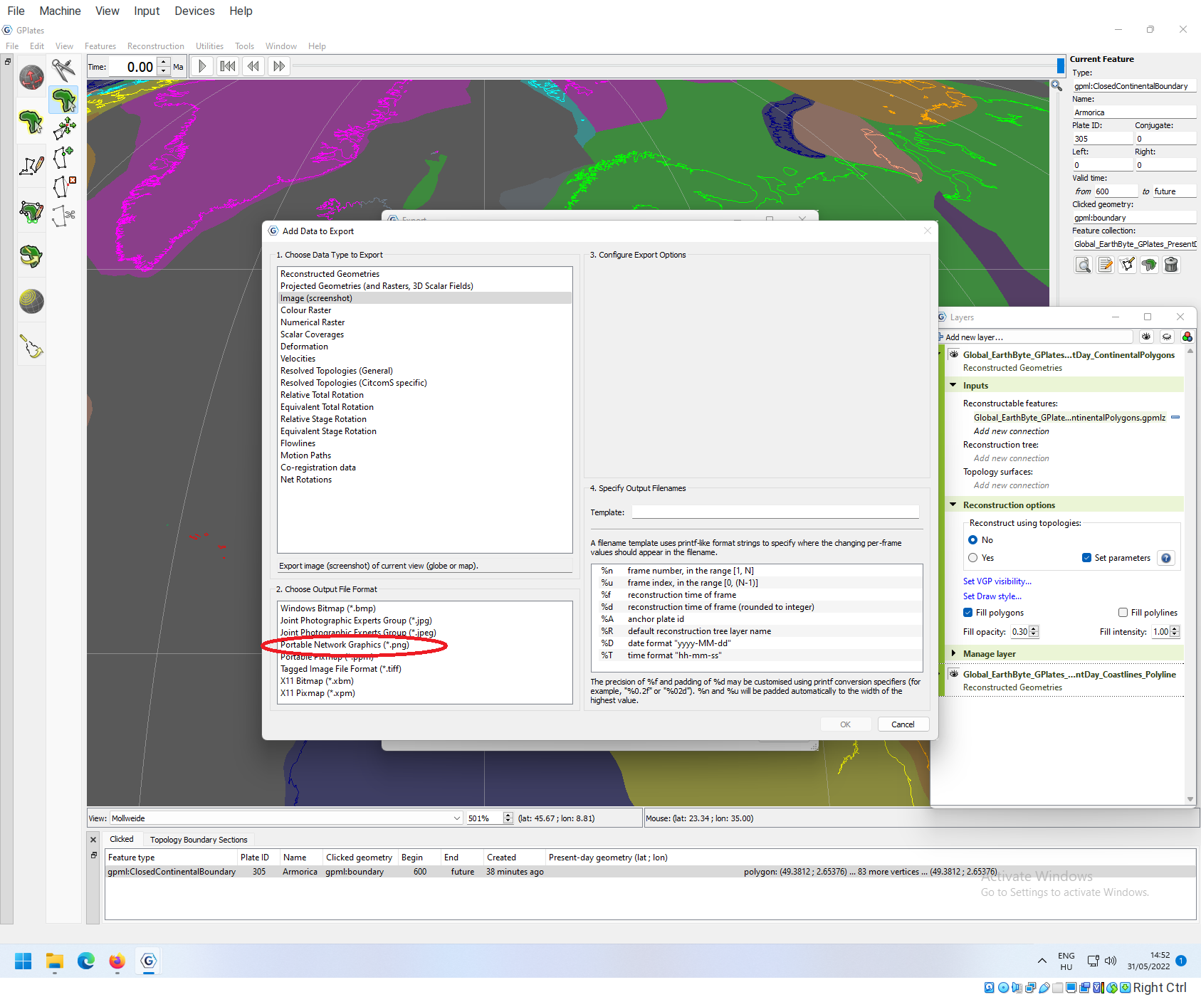
For the sake of this example let’s choose .png (portable network graphics).

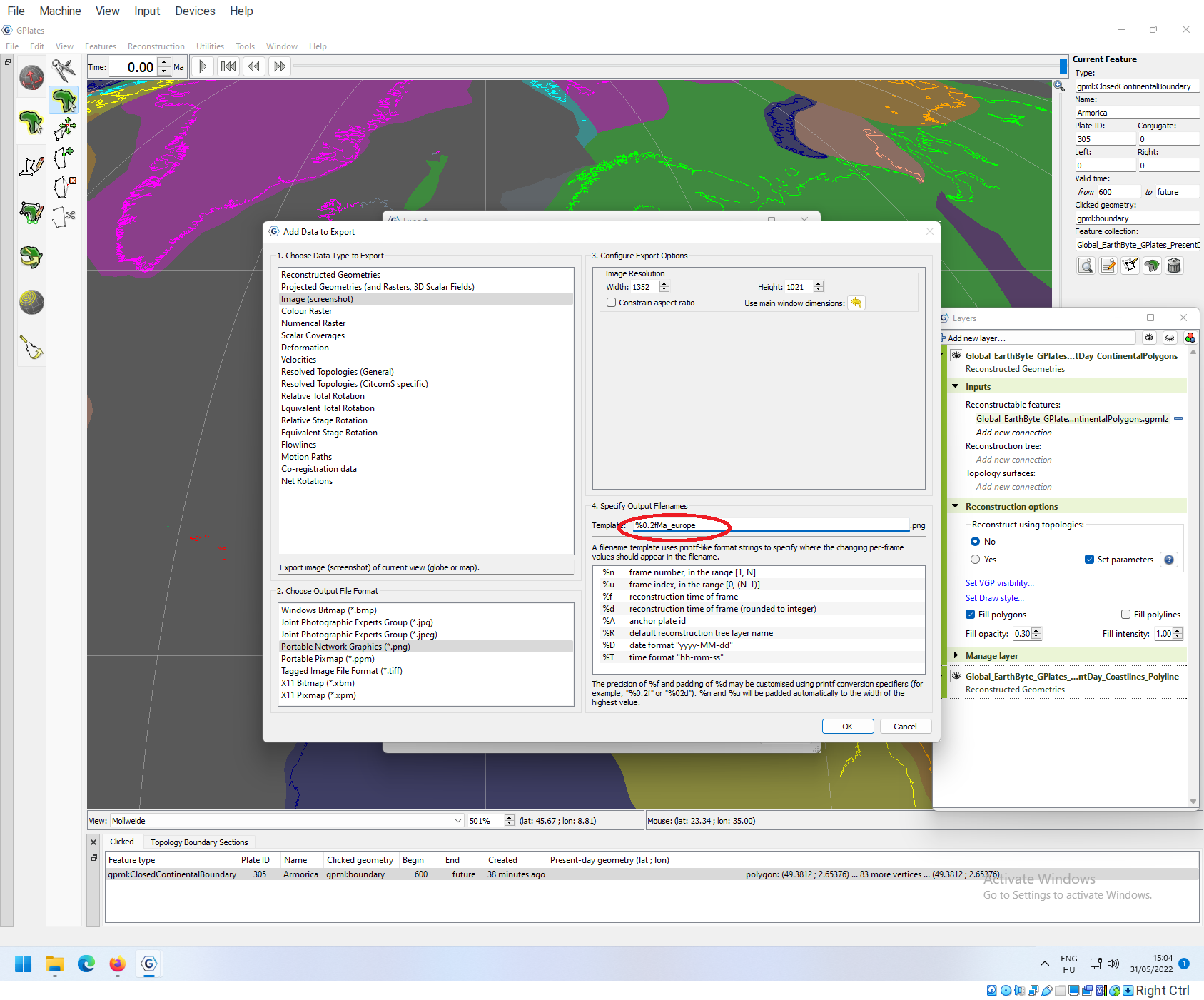
You can then 3. configure the exact dimensions of the image, which, by default will be the same as what you see in the reconstruction window.
Then you can also specify the filename for your reconstruction. This might look somewhat complicated, but it is fairly simple. What you do here, is you write a template filename that has placeholders in it that will change depending on the states of the program. These place holders are listed below the entry field. The default example is image_%0.2fMa, with a .png extension that you can see at the end of the line. This example uses the %ftemplate with an added precision indicator making it %0.2f What this means is: 1. take the current reconstruction time (0.0000 Ma in our case) and 2. round it to two digits. Then this formatted number if pasted into the template, which means that the final name of the file will be image_0.00Ma.png in the end.
To illustrate how this works, let’s change this template up to: %0.2fMa_europe, and click OK.
Now, the new export is added to the list of Export Data.

You can add multiple exports and do them at the same time, if you want. You can also edit existing ones by clicking on Edit….
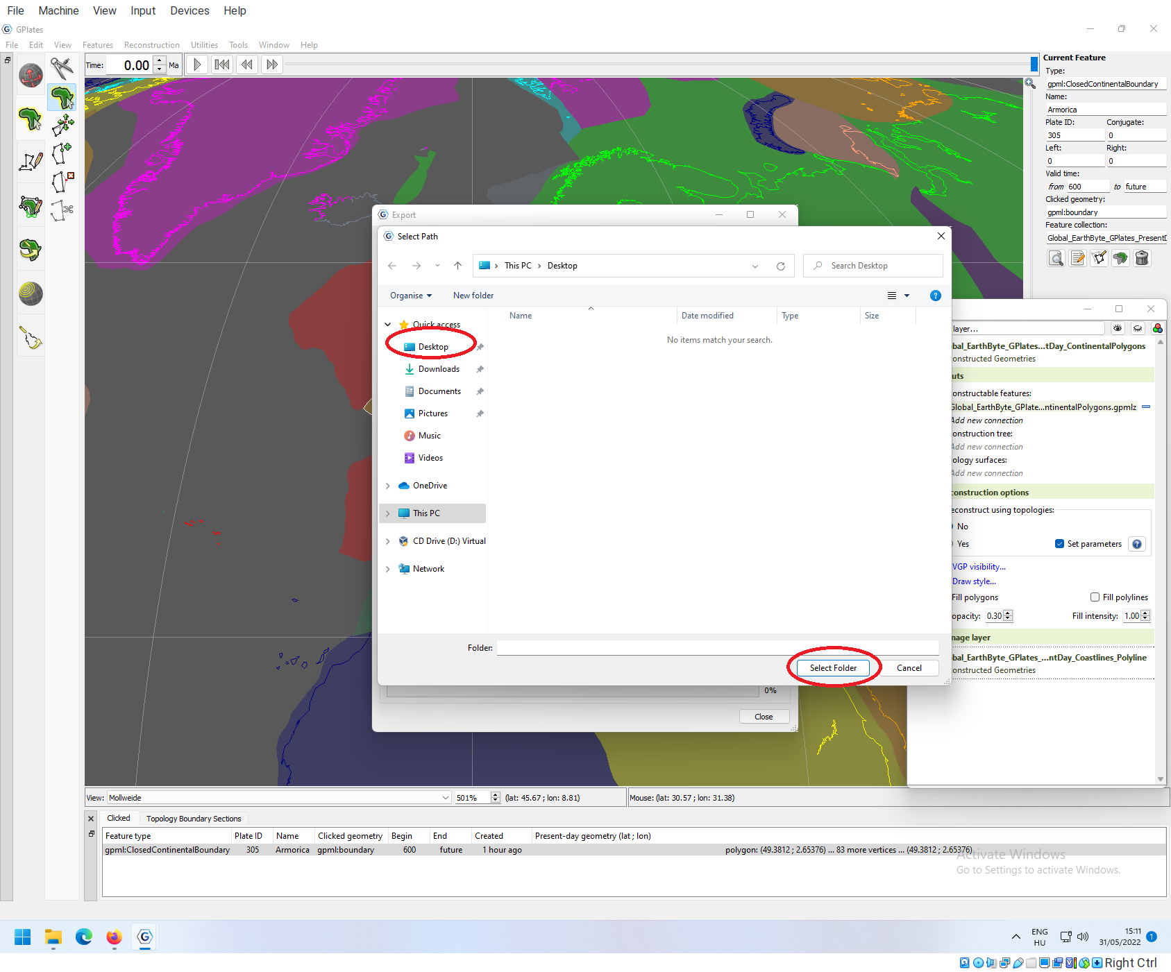
The only thing that remains is to set up where you want to put files that you create. On windows, this defaults to the Documents folder. To change this you have to click on the … next to the Target Directory path:

And select the directory where you want to put the file(s). In this case this is going to be the desktop, click on Select Folder when you are done.
Now we are ready to do the actual exporting. You can click on Export Snapshot and the image will be produced!
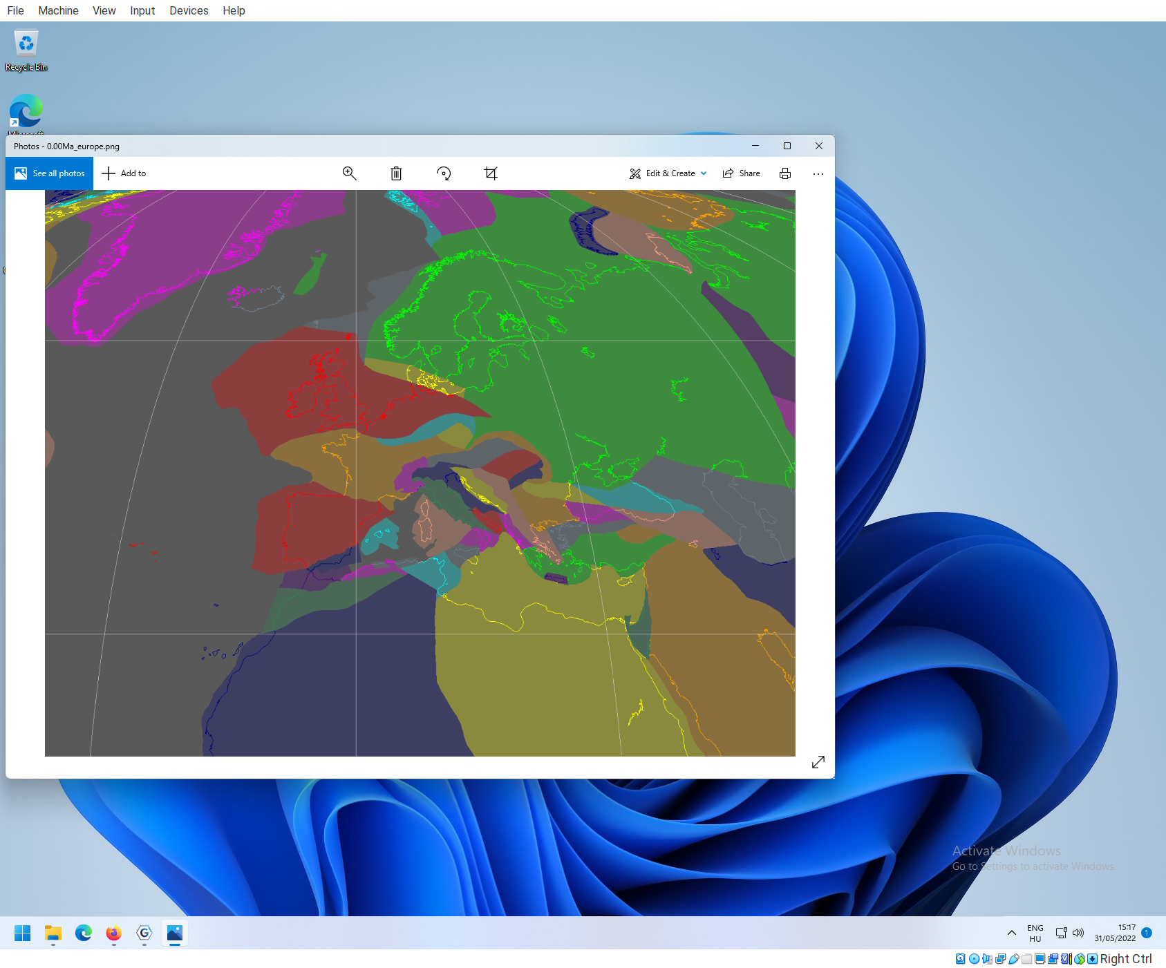
You can close the Export dialog box now, the file 0.00Ma_europe.png is created, and you can open it up in any image editing viewing program.
Unloading features
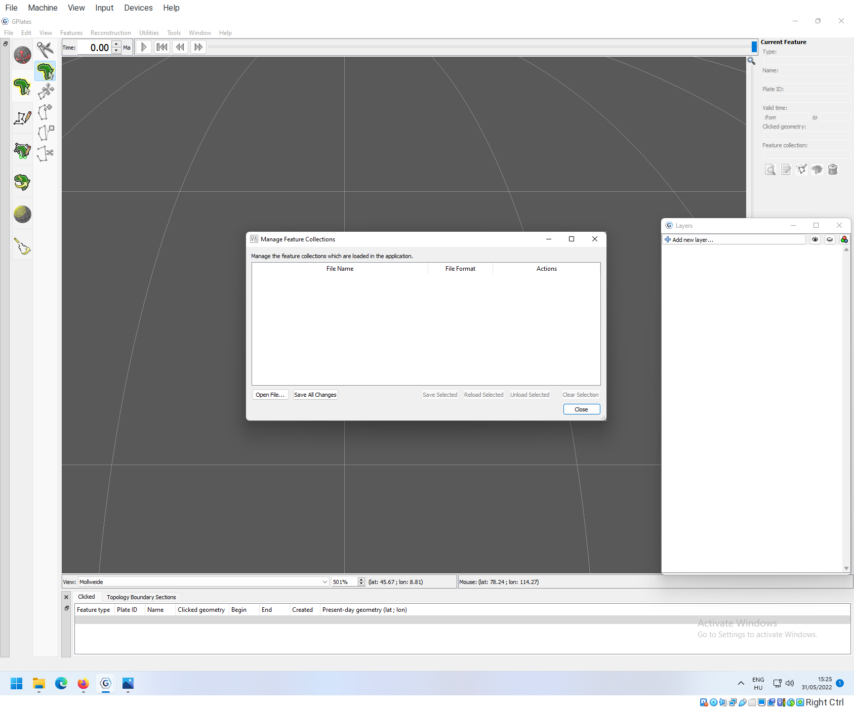
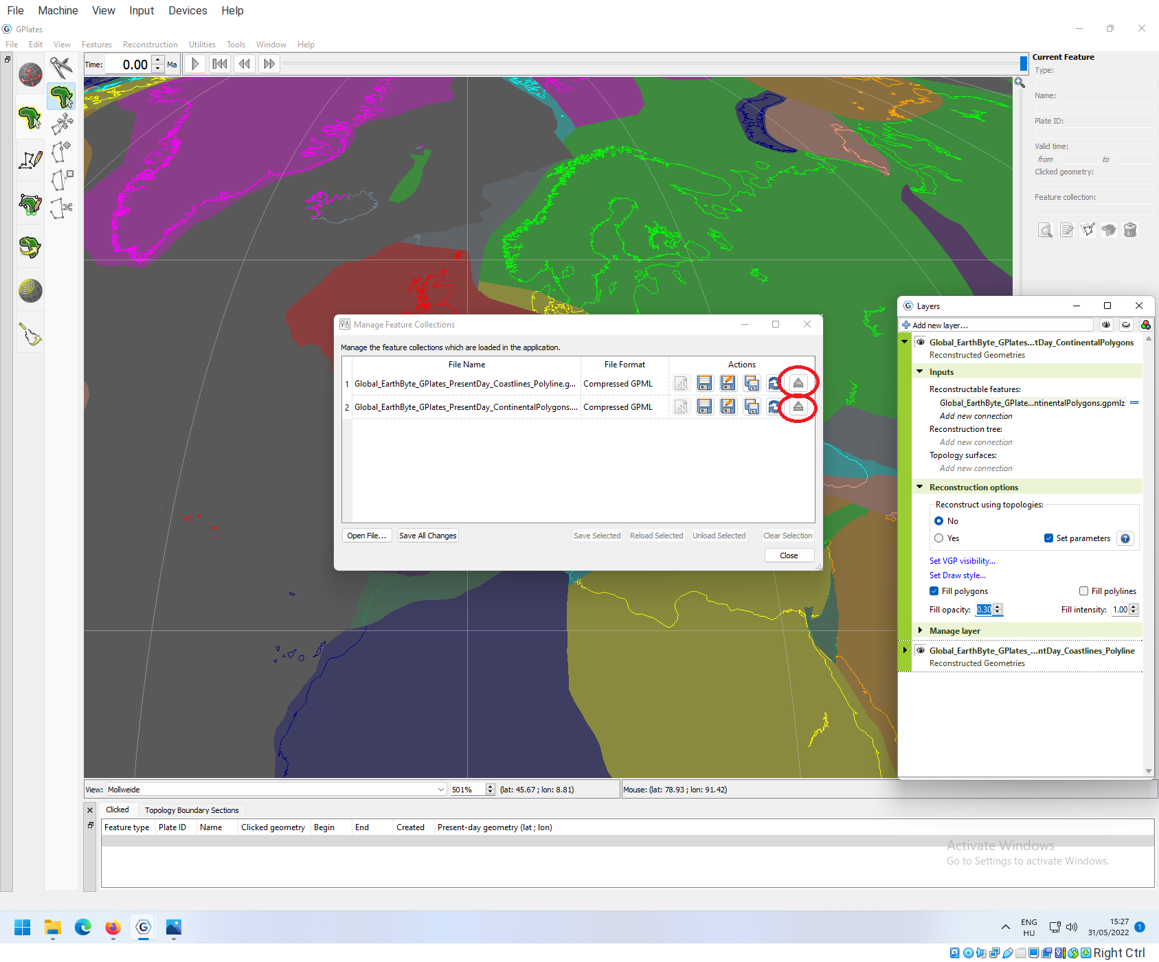
Feature collections can be imported not only by going to File->Open Feature Collection…, but also with the feature manager. If you go to file, you will also see an entry called Manage Feature Collections.
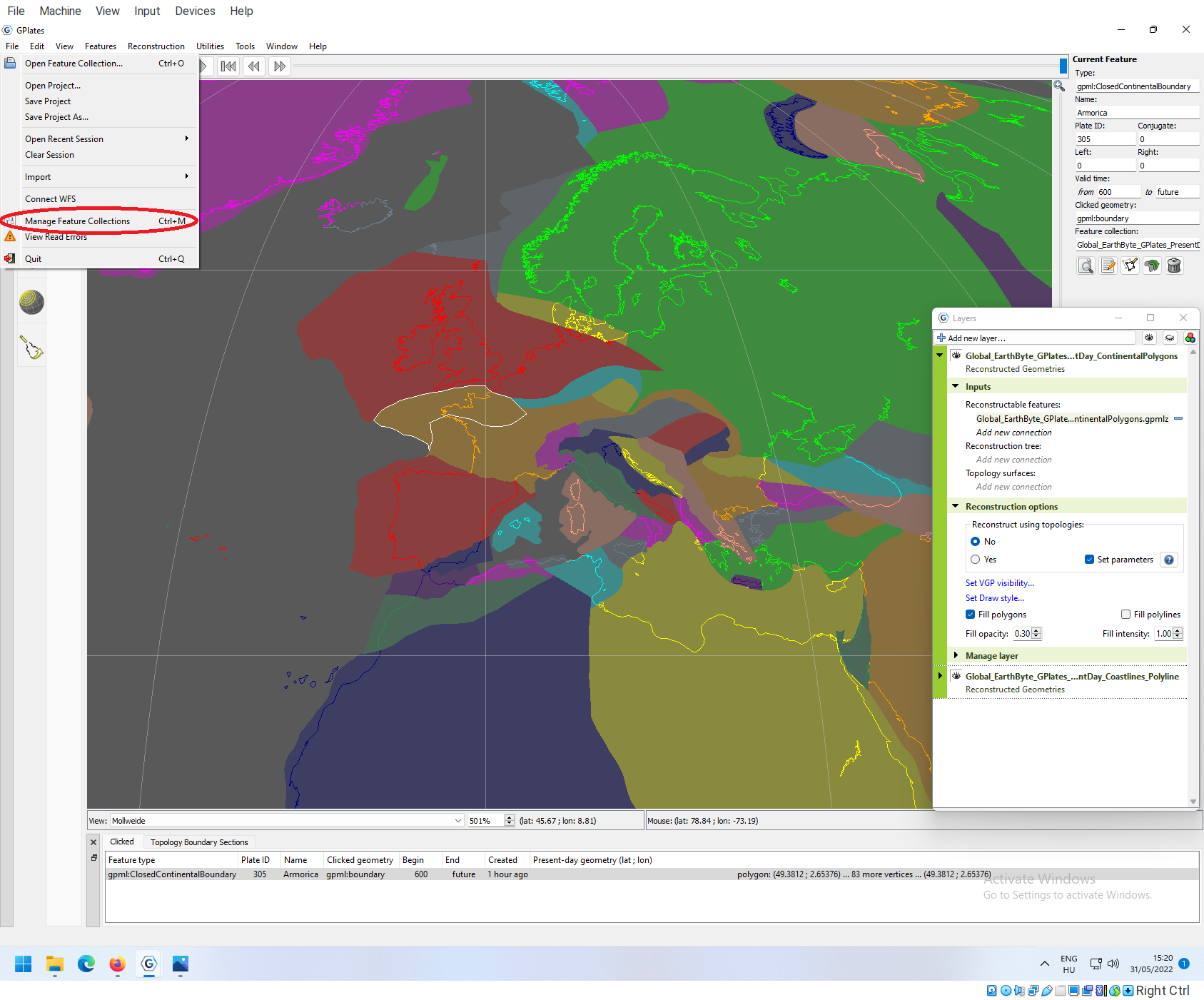
If you click on it, a new window will appear, that lets you to load (Open file…), Save (Overwrite changes in the original files) something that you have changed, or to Reload files. It also allows you to get rid of features from the current workspace.

To get rid of the two feature collections that we have loaded, click on the Unload buttons (last symbols).
This will effectively reset your workspace to the starting state.