Time-dependent rasters
Other tectonic reconstructions
There are two other tectonic reconstructions that come bundled with GPlates.
- The model of Merdith et al. 2021
- and the PALEOMAP model of C. Scotese.
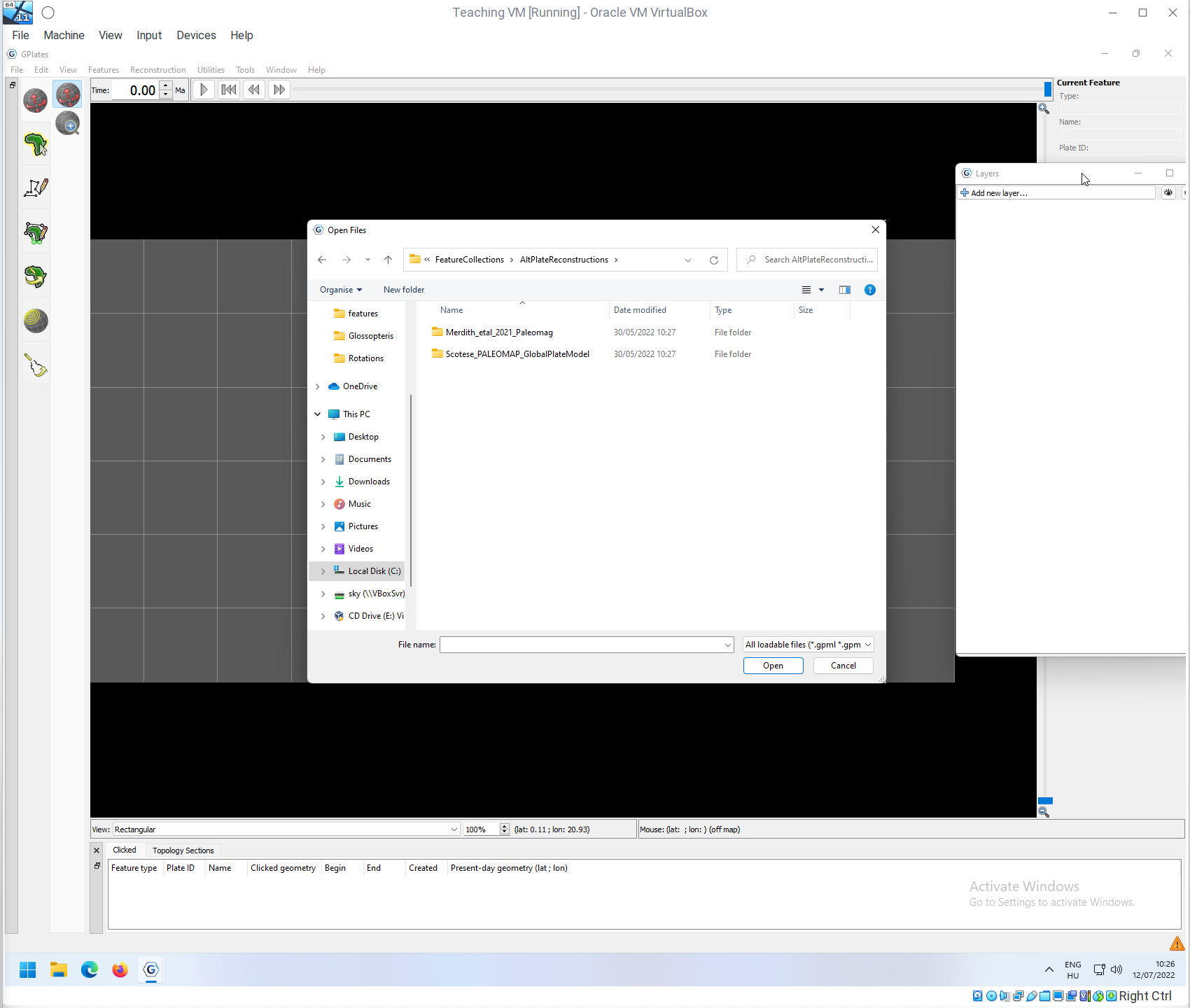
Feel free to explore these models, they are in the GeoData / FeatureCollections / AltPlateReconstructions directory:
The PaleoMAP model
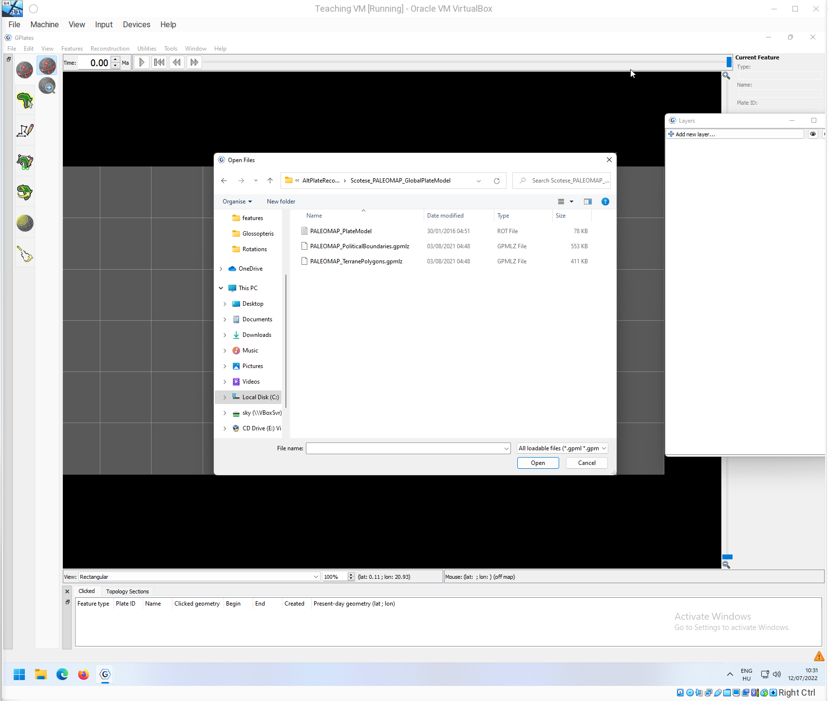
The model of C. Scotese is one of the oldest, and has been developed for decades. You can load in the basic polygons and the rotation file from the directory Scotese_PALEOMAP_GLobalPlateModel. Open PALEOAMP_PlateModel.rot and PALEOMAP_TerranePolygons.gpmlz!
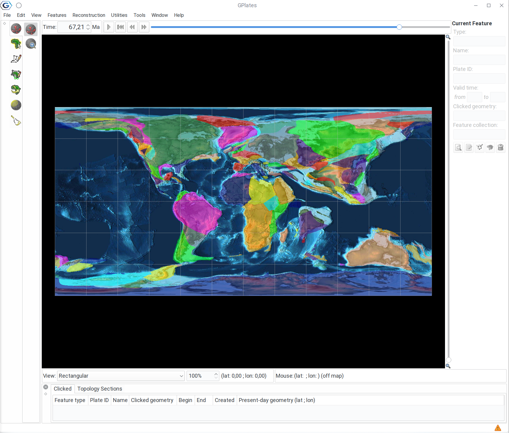
You should see something like, this, for convenience you can turn on the filling of polygons
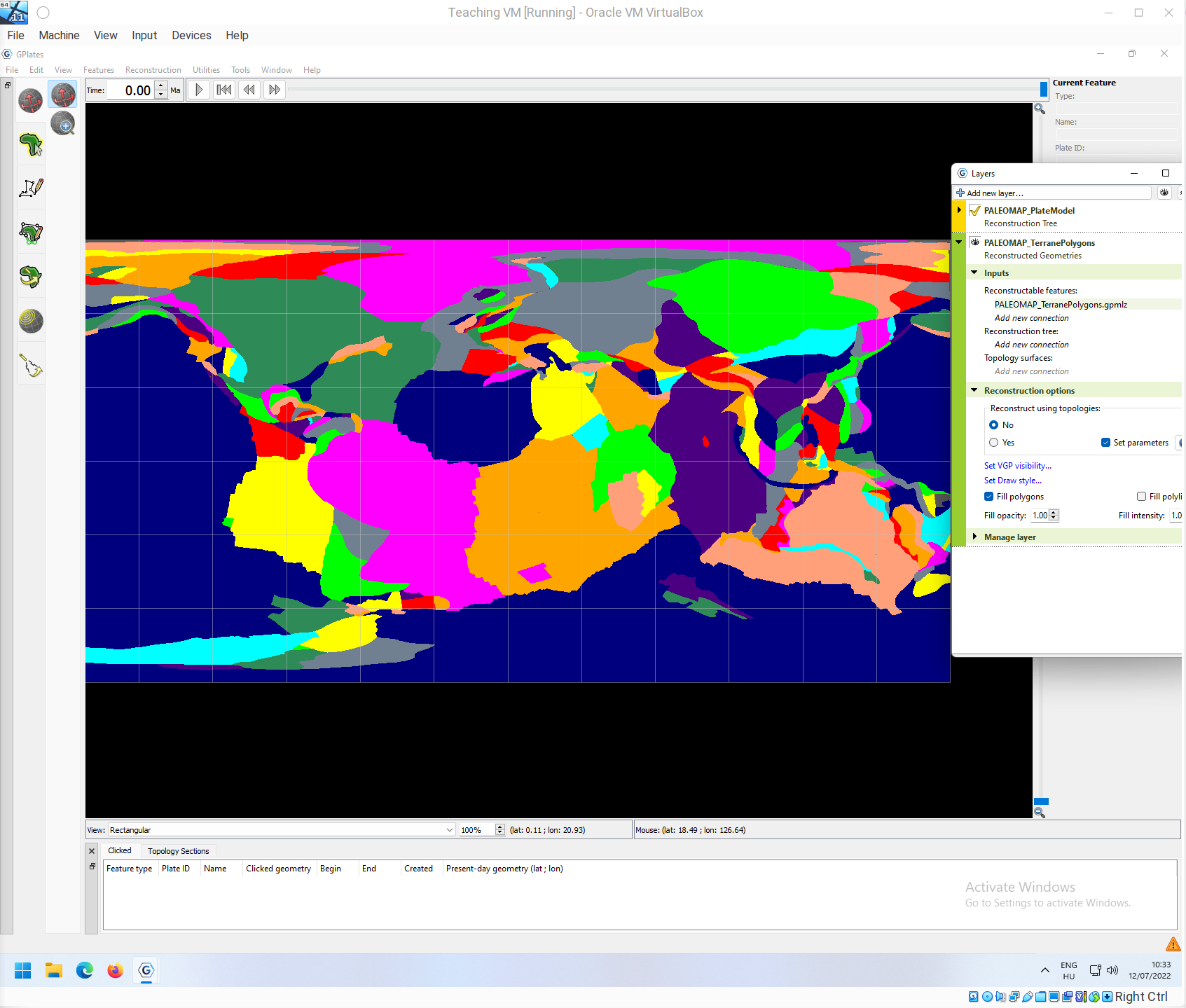
As you can see, the polygons include the oceanic floor by default - however only for the present-day. If you move back in time, the reconstruction tree will already move the polygons, and for convenience, the oceanic floor is not shown.
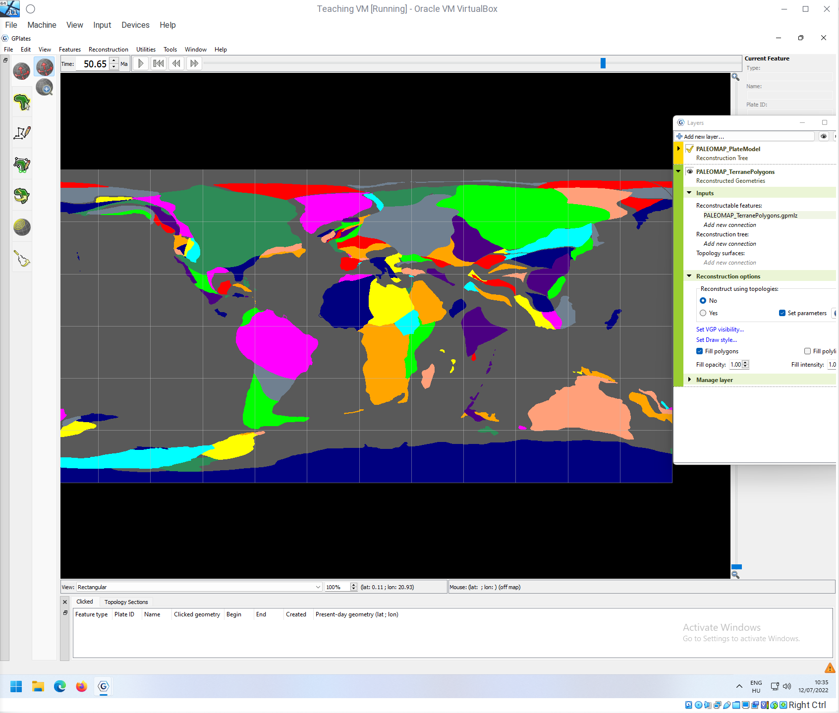
This model goes way back in time… and there is a lot of resources built using this model - for instance reconstruction of topographies, which are time-dependent rasters.
The PaleoMAP PaleoDEMs
Using the plate tectonic reconstructions, present-day topography and timing of events in Earth history, C. Scotese created a set of reconstructions of the Earth’s topography since the Cambrian. These are the so-called paleoDigital Elevation Models.
These can be downloaded either from this link or from the official page of the DEMs here. Go on, and download the zip file!
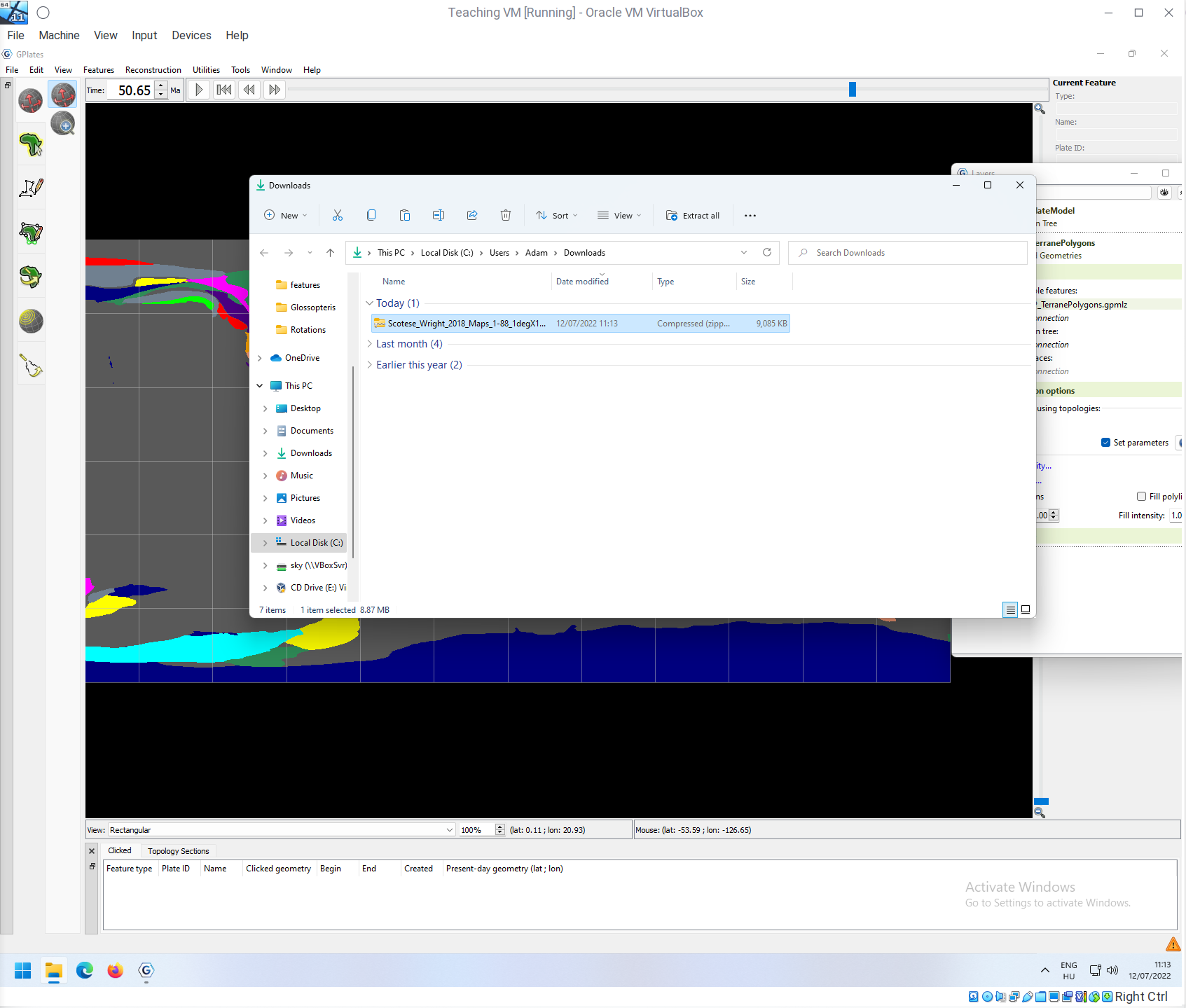
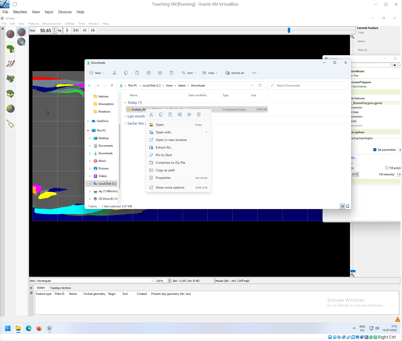
Uncompress this zip file! In Windows 11 you can do this by right-clicking on the zip file in the Windows Explorer and clicking on Extract All!
The default destination should be fine:
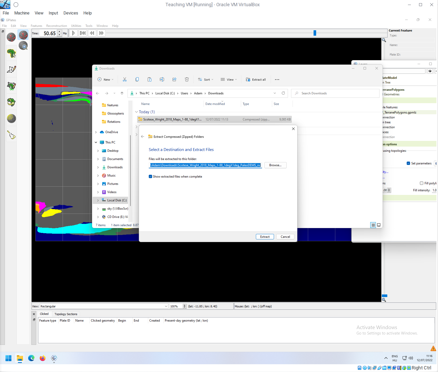
click on extract! This wil create a new directory and put all uncompressed files there.
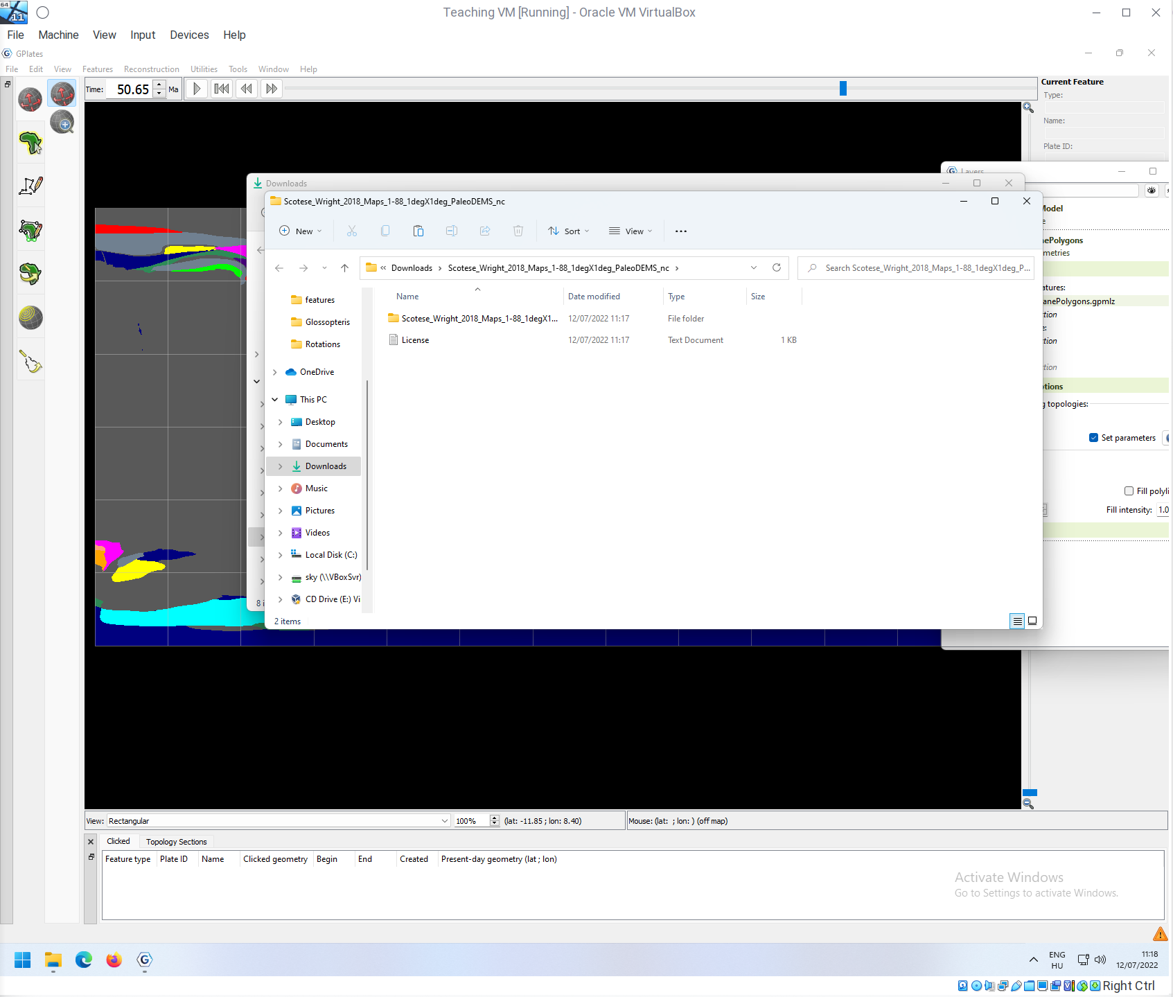
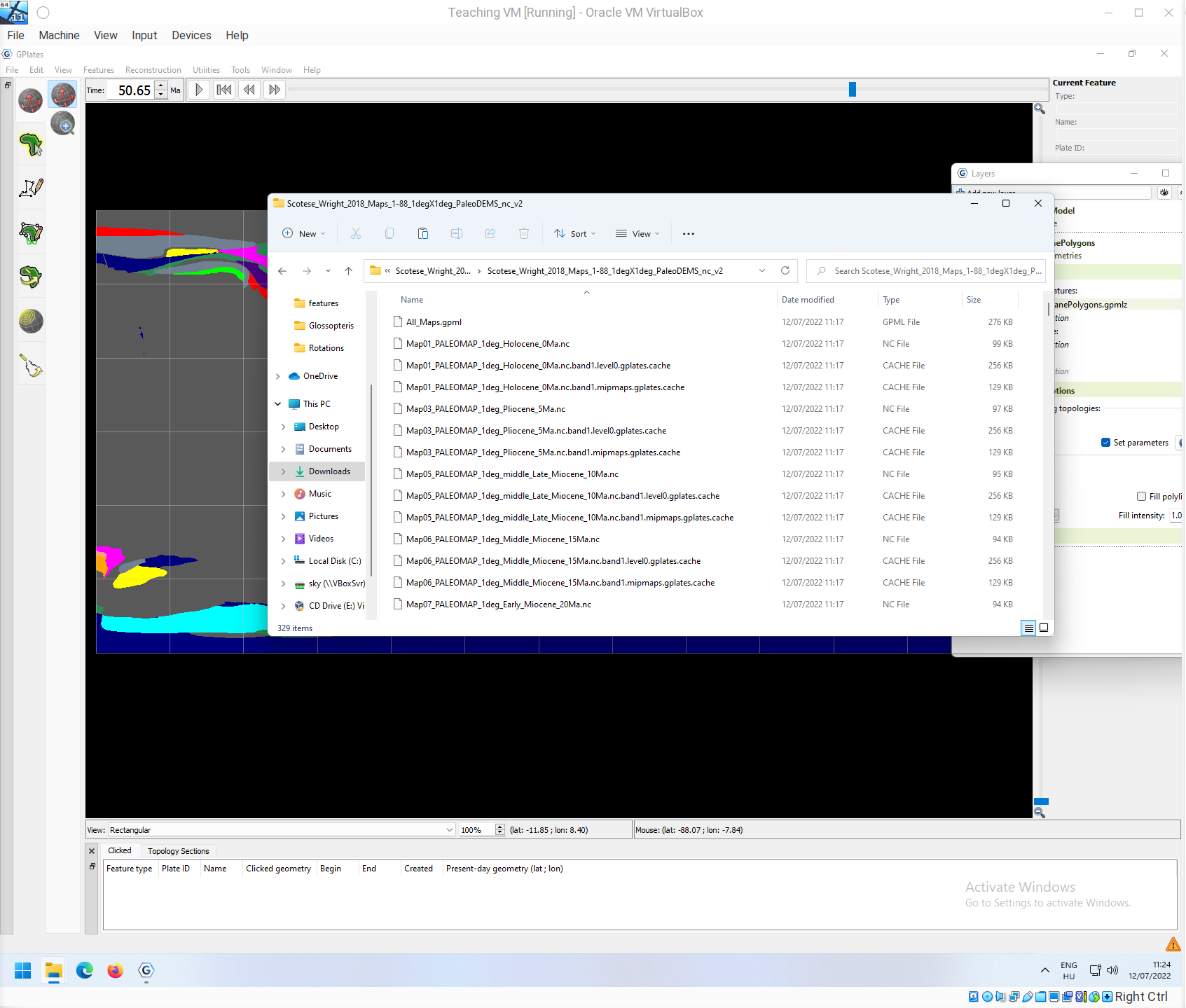
If you go into this directory, you will see a a list of files with .cache and .nc extensions. The .nc files (NetCDF files) include the actual map data. This is a standard binary file format, which is frequently used to store multidimensional (e.g. climate) data.
To import these, go to Gplates and go to File -> Import -> Import Time-Dependent Raster!
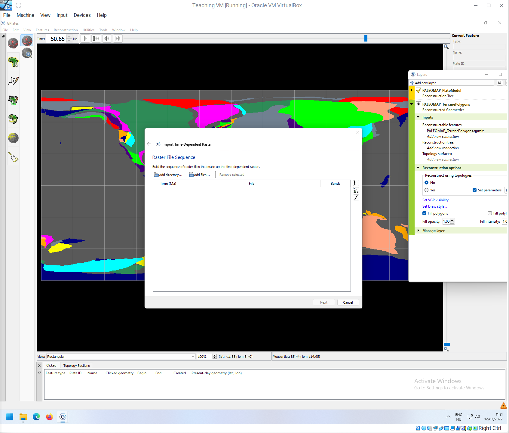
Here you need to specify the directory where all the different raster files are. Click on Add directory…!

This opens up another dialogue window, where you can specify the directory where the NetCDF files are. Navigate to that directory!
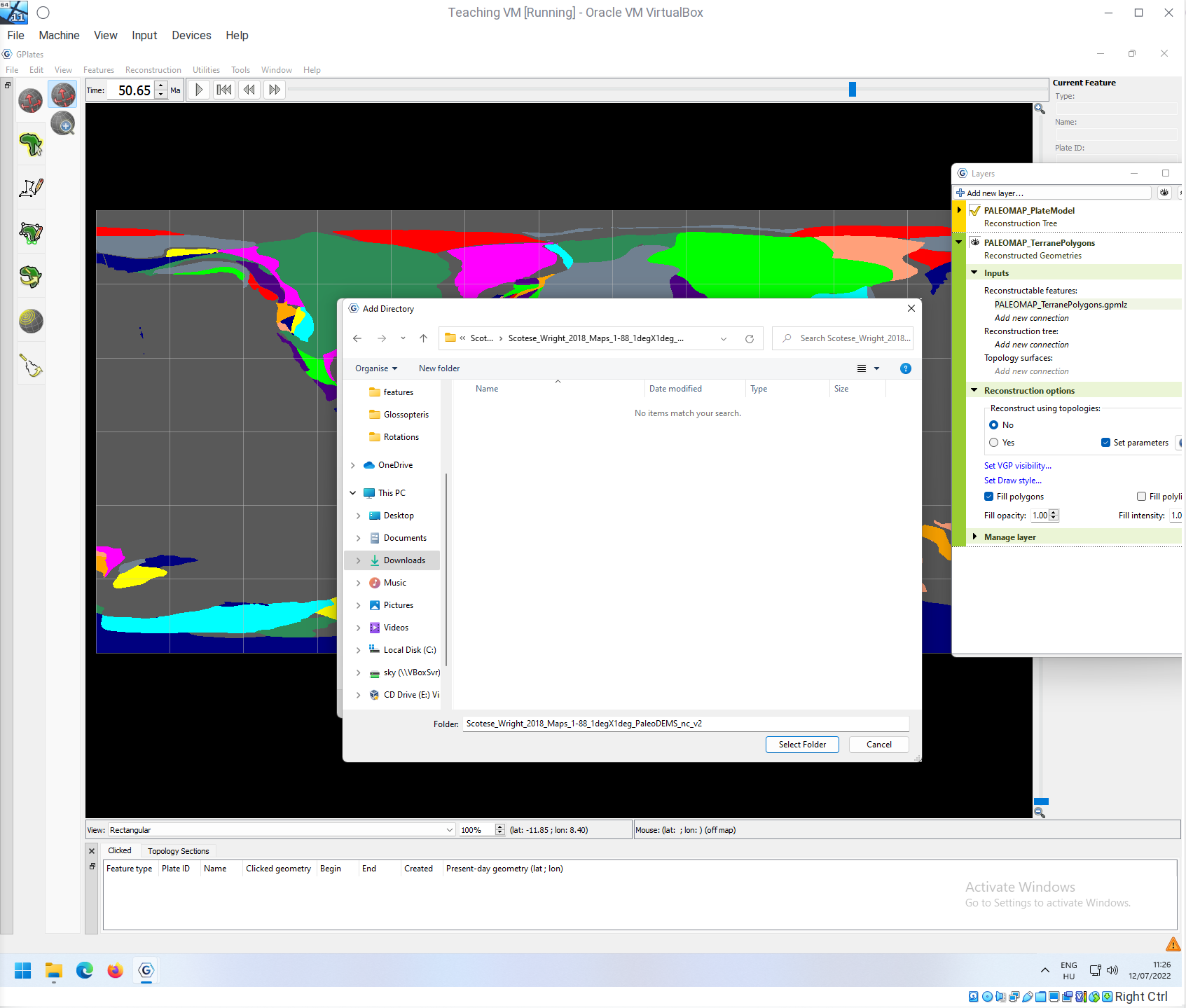
Note that you will not see anything in this directory, because the display filter is set to directories/folders. When you know that you are in that directory where the .nc files are, click on Select Folder!
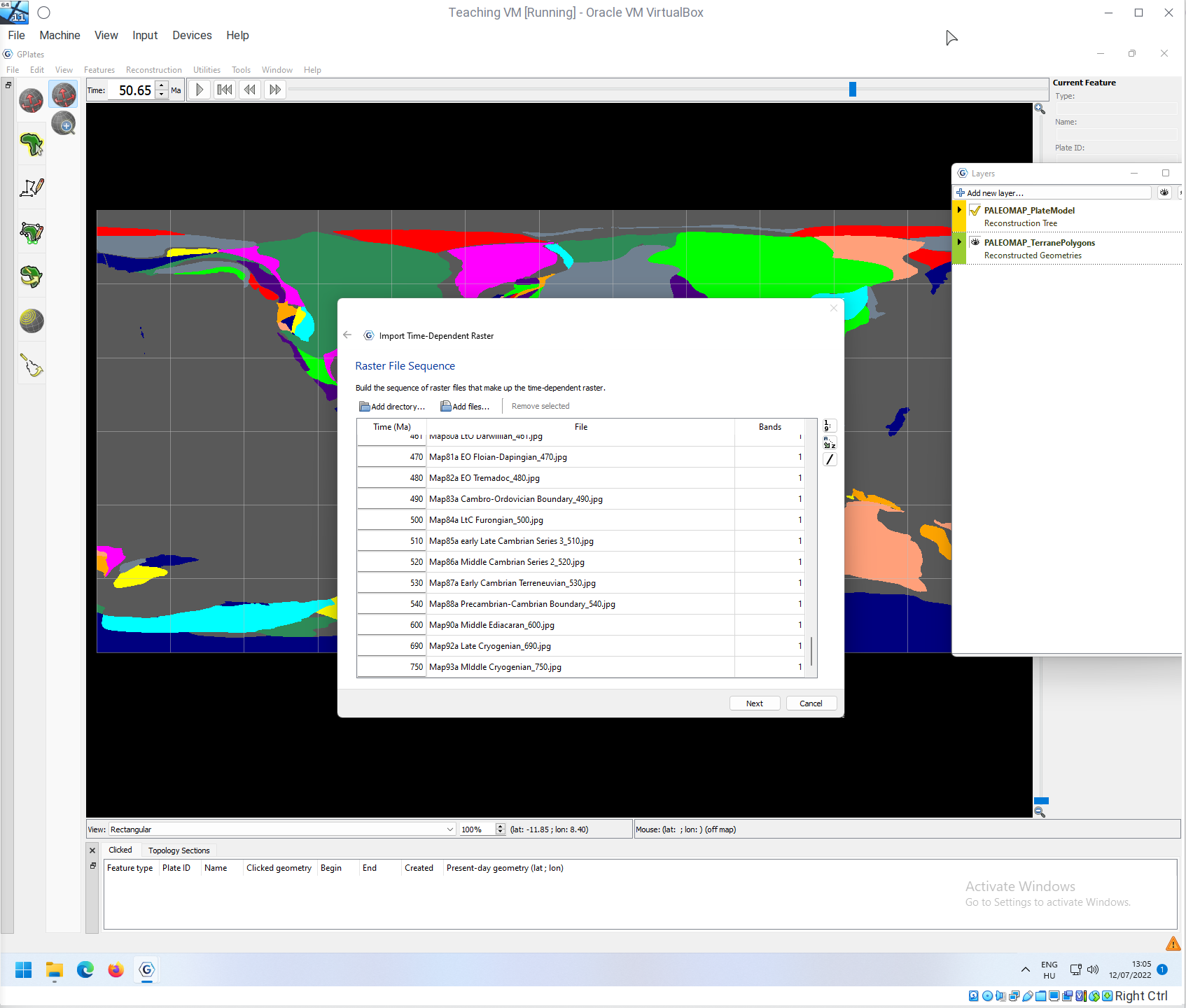
This will jump back to the previous - now populated - window:

Note that there is a table in the middle, with three columns, with information filled in automatically:
- Time (Ma): Based on the file name, what is the age of the map
- File: The actual file name
- Bands: Which raster band will be loaded (for these files this will be the only option)
You can make sure that every file will be processed correctly by scrolling through the entire list. You can manually edit any age or band entry, if necessary. Note that you have one file for every 5 million years. If not, click on Next!

Then you have the option of choosing a name for the band that you are importning. Natively the .nc files have numbered bands, but you can name this, in any way you want/need. The default is fine, so you are welcome to click on Next again.

The normal way of importing such data is by Creating a new Feature Collection (default, shown here). If you have an appropriate already existing feature collection, you can also put the newly loaded information there. Click on Finish to continue!
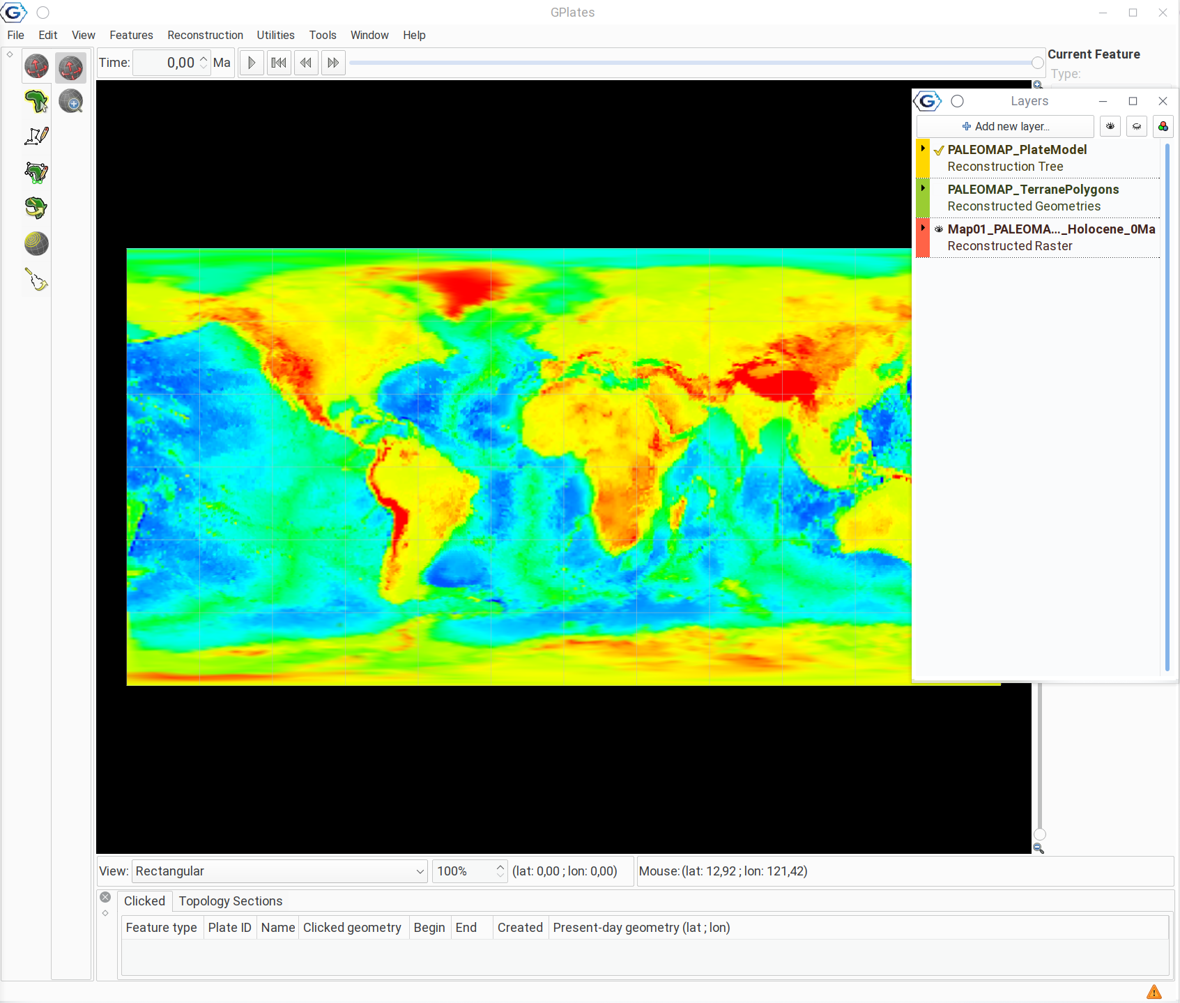
If you have the Plate polygons loaded like in the example, then you will see a heatmap appearing in the background:
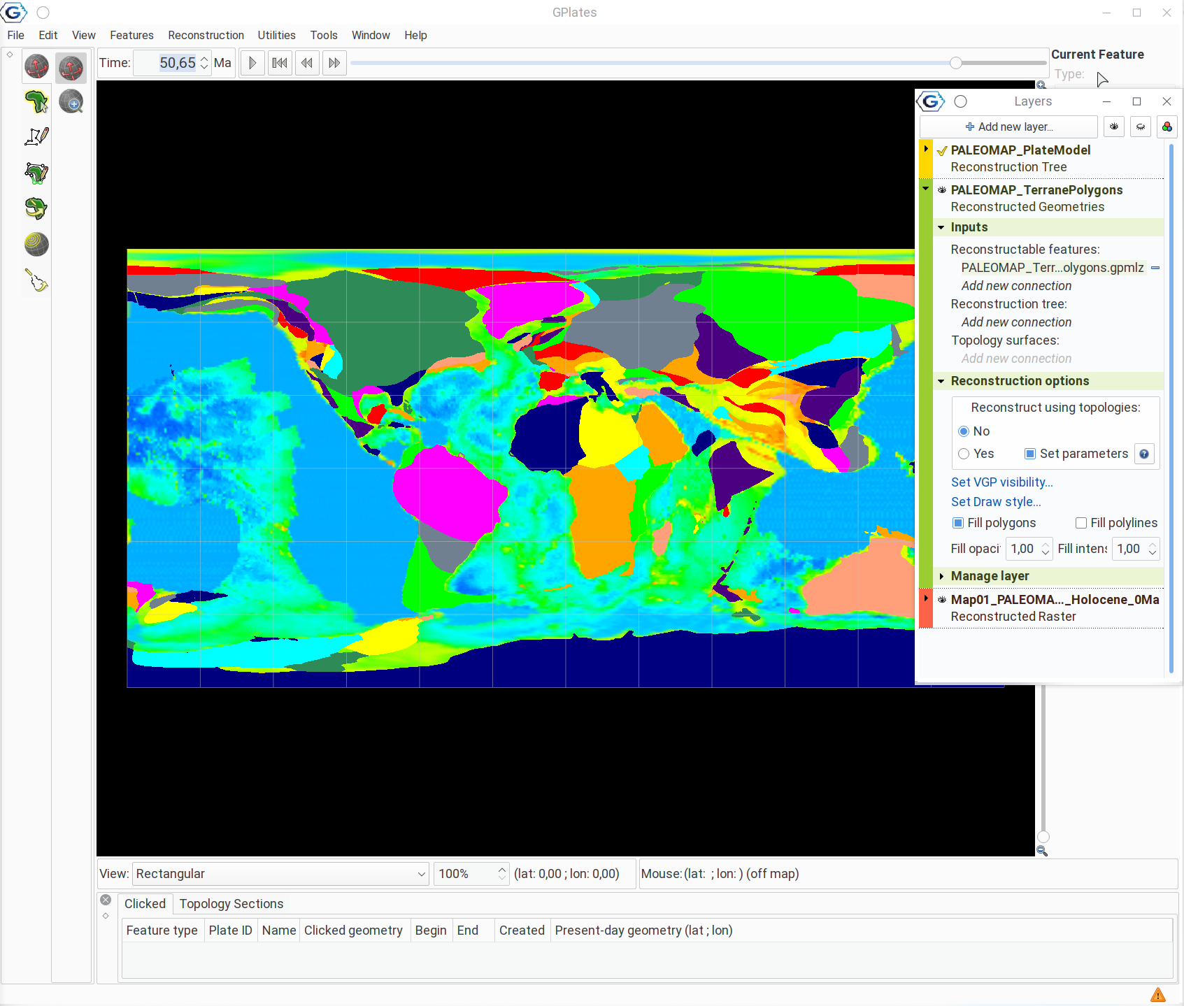
Let’s see what we have really got here. Go to 0Ma (present-day) using the time controls, and turn off the visibility of the TerranePolygons feature! This is what you should see or something similar:
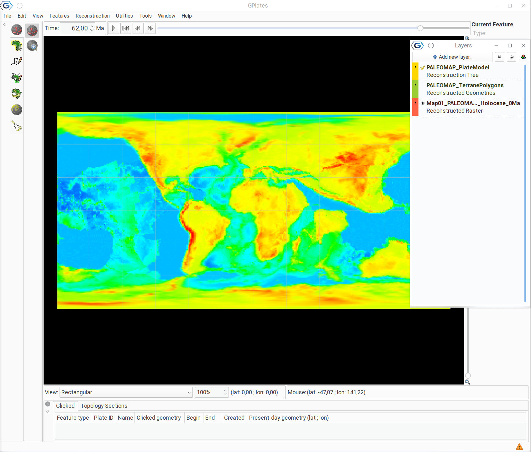
This is the topography of present-day Earth. If you move back in time to say 150Ma (Jurassic/Createceous boundary), the raster will change to the reconstructed conditions at 150Ma:
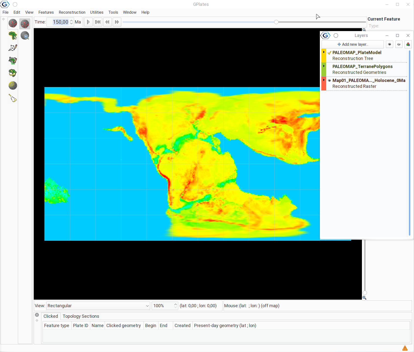
If you hit the play animation button next to the age-input field, you will see that the map jumps at every 5Ma mark. Note that the homogeneity of the seafloor is decreasing as you approach the present day (we don’t have fossilized in-situ seafloor from the first half of the Phanerozoic).
This is because what you see are snapshots: time moves continuously but the maps don’t. This is a temporal limit of this reconstruction.
However, you can see, how this matches the underlying the plate polygons that were used as a baseline for creating these, if you turn on the visibility of the PALEOMAP_TerranePolygons again, decrease the Fill opacity to 0.5.
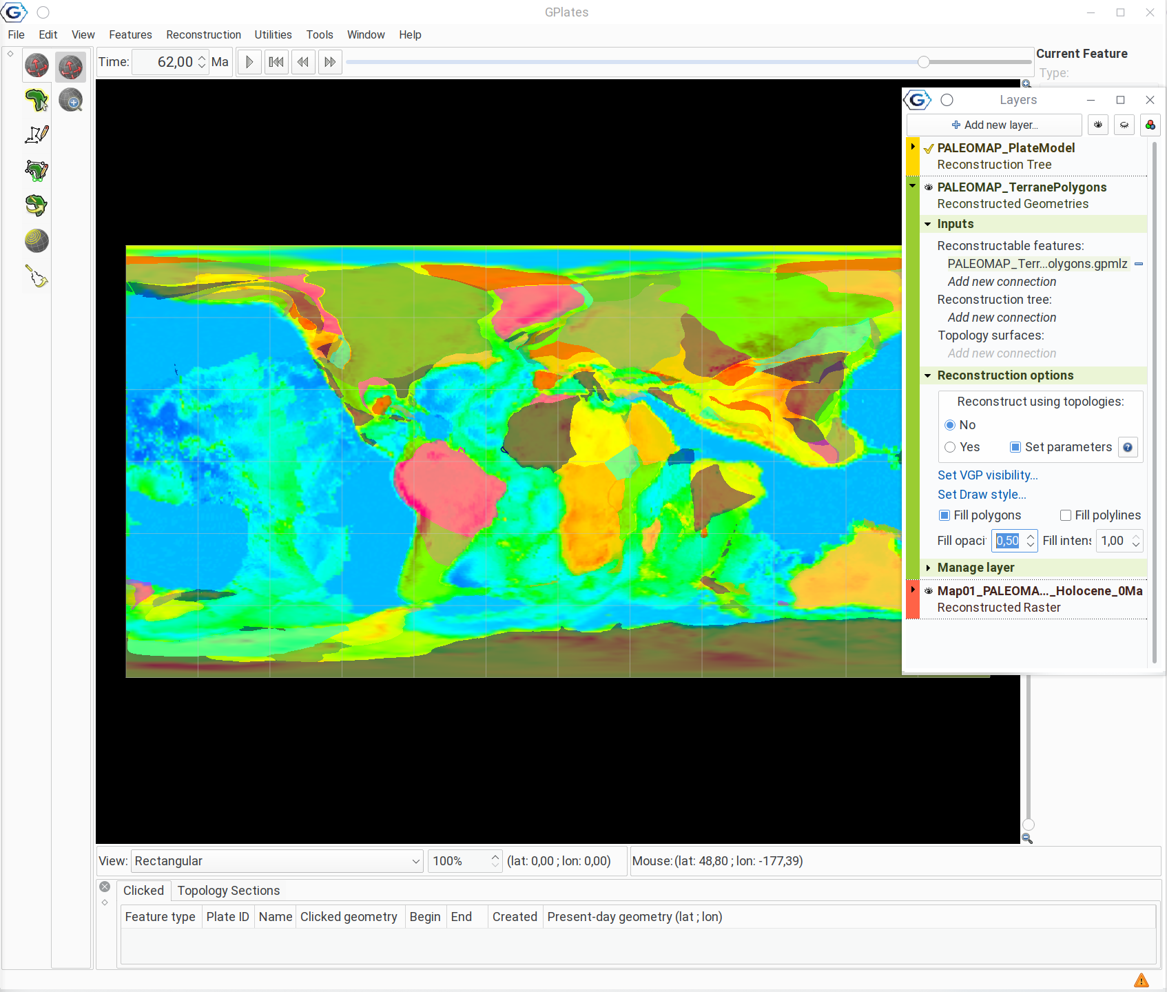
If you hit the play button now, you should see that the plate reconstructions have much finer temporal resolution, they move much smoother than the underlying maps. Also note that two are aligned only at the nominal ages of the topography reconstructions (ages that are the multiples of 5 Ma), and are somewhat misaligned in other times. This is good to know when you are saving maps like this with the Export feature.
Note that you can also customize the raster heatmap palette here as you could do it with the single rasters.
The match between the high topography-areas and the plates is far from perfect. Some plates have relatively low eleveation (e.g. submerged continental plateaus). Sometimes we just don’t know much about the exact depth of the sediment deposited on the a plate at the reconstruction time, and there are also some geometric-extensions that must have been there, even though today they are not in their original position anymore (e.g. continental slopes). The reconstrution of paleogeography is a never-ending quest. In any case, you can learn more about these here, from the original booklet coming with the reconstructions.
The PALEOMAP PaleoAtlas
This is very nice, but it is not that visually appealing. For this reason (actually before this), C. Scotese published a set of rendered images called the PALEOMAP PaleoAtlas, which is a similar set of images. You can also download it from here.
The process to load these is exactly the same as for the PaleoDEMS.
- Download and uncompress the zip filem
- Import as time-dependent rasters.
The rasters are .jpg files in the PALEOMAP PaleoAtlas Rasters v3 directory.
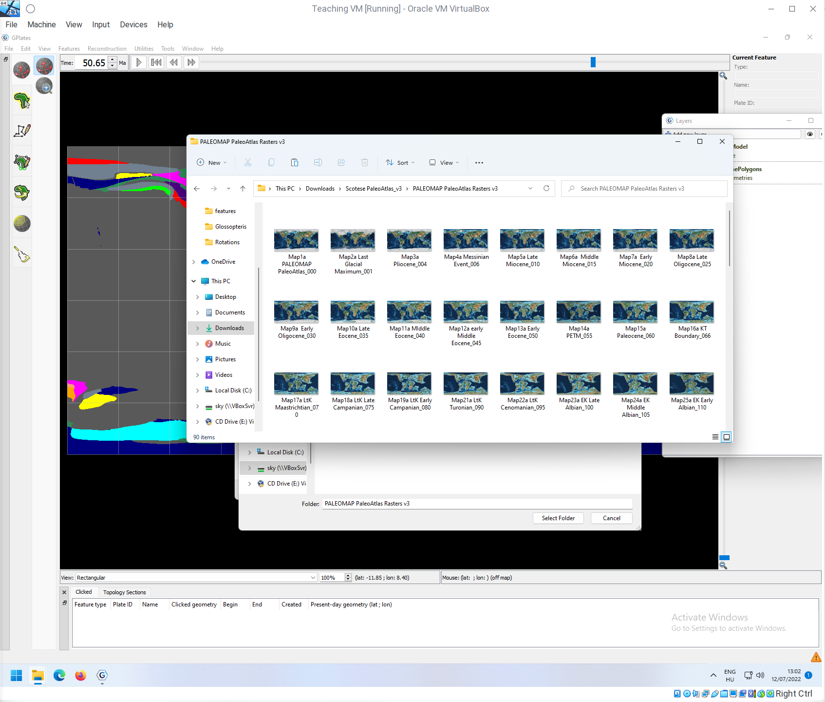
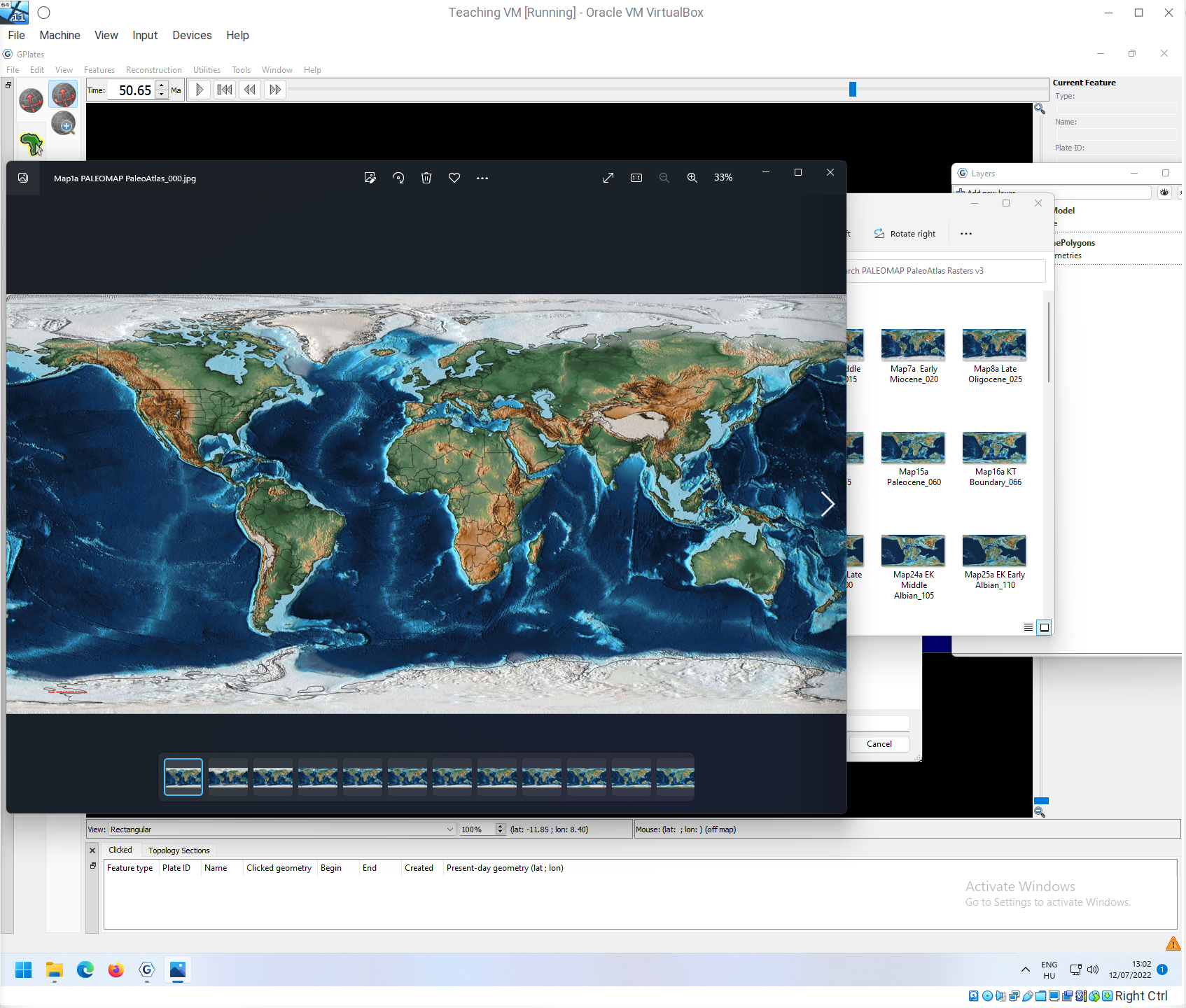
The information is readable in any image-viewer program, but it will not be georeferenced. You can also open these files with a regular photo/image viewer,
This is the directory that you need to open as a time-dependent raster, as above. Note that it takes a bit longer to open this directory, since the data need to be cached (which was done in the .cache files in the case of the PaleoDEMs):
The rest of the steps should be the same, except that now you also have to approve the actual Georeferencing:
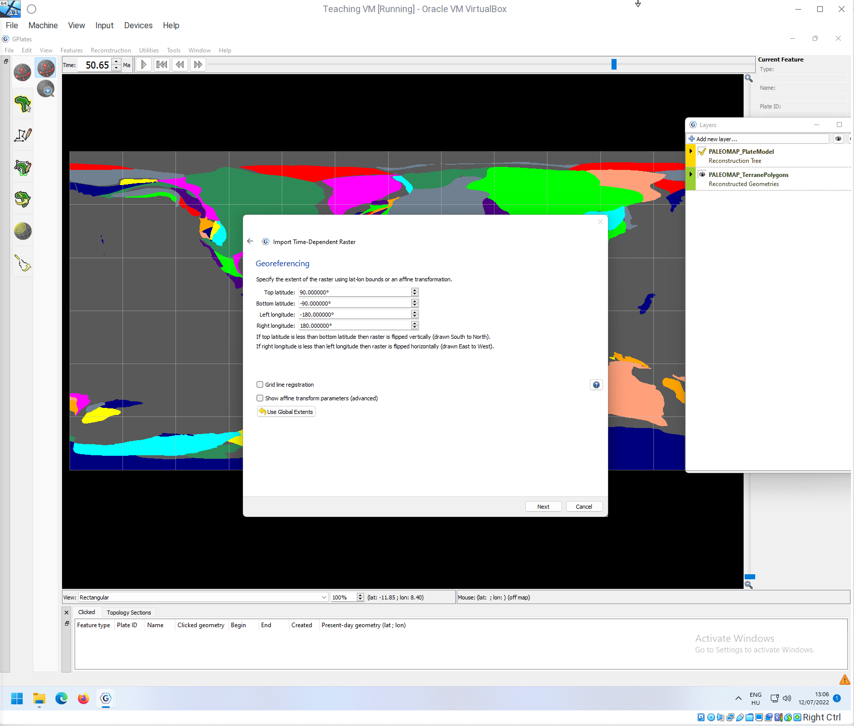
This is because you are opening regular image files that were produced with software that plots everything in a ready-to-import way, but no actual georeferencing information is included in the files. This is assumed by GPlates, which is in our case the right one. The rest of the importing process is the same as above, but instead of having topography rasters, you have actual images for every 5Ma, which you can see with the plates overlain on top of the reconstructions.
These reconstructions will also move with time (as the PaleoDEMs), and they look quite cool. However, none of these are useful if we cannot put information on these maps, i.e. to be able to reconstruct the paleocoordinates of user-defined present-day coordinates.